Project:Bike Sharing Prediction

Introduction

Data source: hour.csv in Bike Sharing Data Set on Data Science Dojo.

About Dataset: The bike rental dataset contains information on the hourly and daily count of rental bikes in the Capital bikeshare system, as well as corresponding weather and seasonal data. The dataset contains 17 columns and 17379 rows. The original attribute names and definition are shown by the following table:

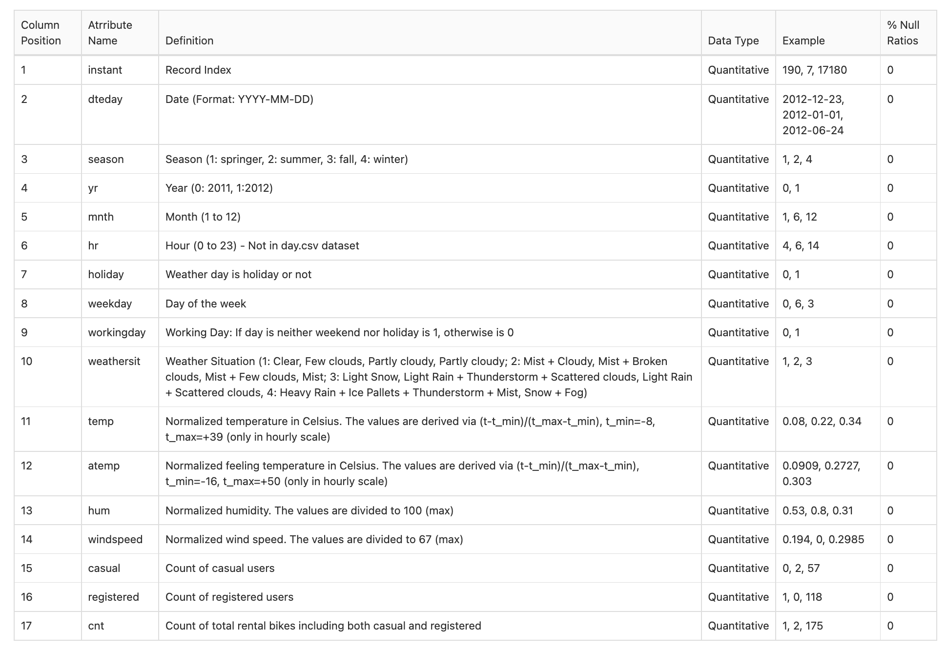
The bike rental dataset contains both categorical and numerical data. Data type shown in the original table is incorrect (e.g. holiday should be categorical), which will be dealt with in the data cleaning section.

Categorical data includes yr, season, month, hr, holiday, workingday, weekday, and weathersit, which can be used to predict the number of rental bikes.

Numerical data includes atemp, hum, and windspeed, and has been normalized to ensure that all values are on the same scale, which is important for linear regression analysis. By using linear regression, it is possible to explore the relationship between atemp, hum, windspeed, and cnt. This can help quantify potential trends or patterns in the data, such as an increase in bike rentals during the comfortable atemp. Additionally, this analysis can be used to identify potential correlations or trends in these relationships.

Data Cleaning

Delete irrelevant attributes:

• dteday: This attribute tells the exact date of each rental, but we don’t need this level of detail. Instead, we choose the season, yr, mnth, hr, holiday, weekday, and workingday attributes to describe the general type of day.
• temp: This attribute tells the temperature of each record. It is highly correlated with the atemp attribute, which tells the feeling temperature. Since both attributes contain similar information, we only need to keep one of them to avoid redundancy and improve the interpretability of the dataset.

Correct data types:

• season, yr, mnth, hr, holiday, weekday, workingday, and weathersit: These attributes are currently stored as numerical values, but they should be categorical data. To improve the interpretability and accuracy of our analysis, we can convert these variables using as.factor() in R. This will ensure that any analysis or modeling we perform with these variables will accurately reflect the categorical nature of the data.

Remove unreasonable values:

In windspeed and hum, there is an unreasonable number of 0 and 1 values, which could be caused by: incorrect interpretation of N/A, rounding up/down decimal places or actually being 0 or 1. Since we can’t decide which of the above is the correct one, we choose to replace all of them with N/A for the moment to avoid contamination of the data.

Clean outliers:

• Numerical attributes (atemp, hum, and windspeed): These attributes contain some extreme values that can be considered as outliers. To clean these values, we first calculates the upper and lower boundary values for each variable using the mean and standard deviation. Any values that are outside of these boundary values are considered outliers. Then we cap the outliers by setting them to the upper or lower boundary value. This would effectively remove the outliers from the atemp, hum, and windspeed columns, improving the quality and interpretability of the dataset.

• Categorical attributes (year, season, month, hour, holiday, workingday, weekday, and weathersit): These attributes may also contain outliers, but in the case of categorical data, outliers are usually defined as values that have a frequency (i.e. the number of occurrences) that is lower than a certain threshold. Here we choose 100(~0.5%) as our threshold, meaning any categorical values with fewer than 100 occurrences will be removed.
  Overall, these steps will help improve the quality and interpretability of the bike rental dataset, and enable us to perform more accurate and reliable analysis.

Data Analysis

Part 1: Basic Statistics

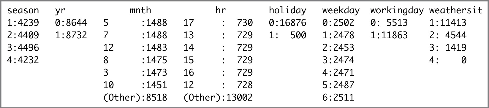
After data cleaning, summaries of the dataset are as follows: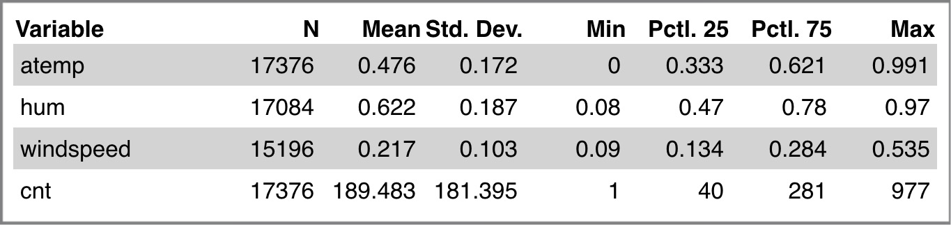

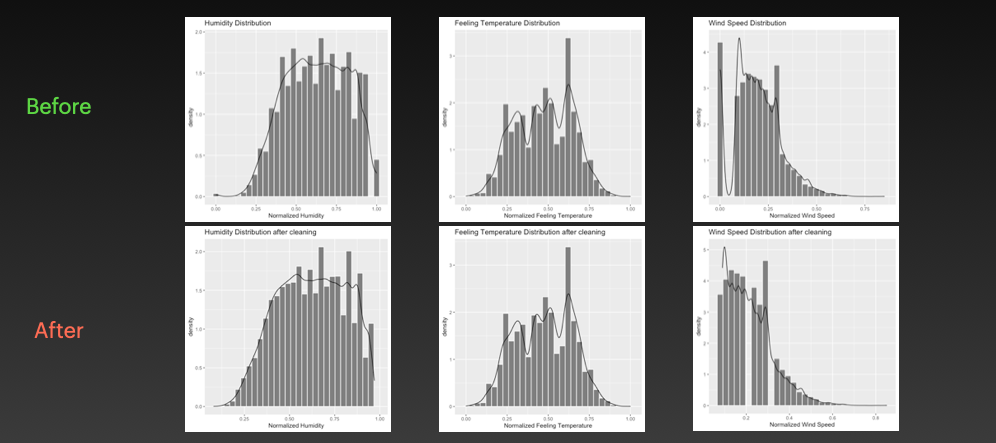
Distributions of the data values are as follows: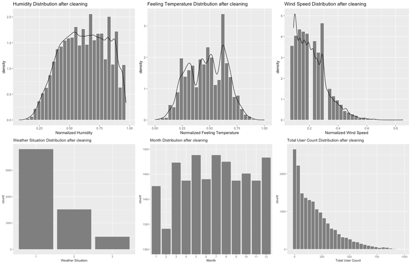

From the plots we can conclude:

• Wind speed distribution is right-skewed.
• Humidity distribution is left-skewed.
• Feeling temperature distribution is symmetrical.
• User count distribution is L-shaped.
• There are a lot more weathersit = 1 rows than the others.
• There are relatively similar number of rows for every month.

Part 2: Exploratory Data Analysis (EDA)

For this part, we look into the basic correlation between every other attribute and cnt. Plots are as follows: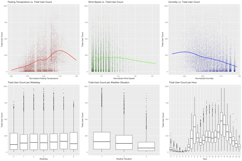

From these plots, we can conclude:

• Feeling temperature generally has a positive impact on total user count.

• Humidity has a negative impact on total user count.

• Wind speed doesn’t seem to have a significant impact on total user count.

• Weekday doesn’t significantly impact user count, but weather situation and hour do.

• There are generally a lot more users in weathersit 1&2 and hr 8&17, representing peak hours in good weather.

Part 3: Hypothesis Testing

After data cleaning and EDA, we identified three interesting factors affecting user count (cnt): Hour in a day (hr), Year of data (yr) and Day in a week (weekday). So we need to look further into the difference they make. We conducted hypothesis testing to do this.

For all following tests, we set the level of significance at α = 0.05, meaning we accept a 5% chance of making a Type I error.

Testing hr

Question

The mean of cnt is 189.483. Is there a significant difference between cnt from the first hour of the day (hr = 1) and 189.483?

Setting up the hypothesis

This is a two-tailed, one-sample t-test.

• Null Hypothesis: mean(hr =1) = 189.483, cnt from the first hour of the day is not significantly different from 189.483.
• Alternative Hypothesis: mean(hr =1) ≠ 189.483, cnt from the first hour of the day is significantly different from 189.483.

Test result

The resulting p-value, p < 2.2e-16, is magnitudes smaller than α, so the null hypothesis was rejected.

Conclusion

cnt from the first hour of the day is significantly different from 189.483, the mean of all cnt, meaning hour of the day has a significant impact on user count.

Testing weekday

Question

The mean of cnt is 189.483. Is there a significant difference between cnt from the first day of the week (weekday = 1) and 189.483?

Setting up the hypothesis

This is a two-tailed, one-sample t-test.

• Null Hypothesis: mean(weekday =1) = 189.483, cnt from the first day of the week is not significantly different from 189.483.
• Alternative Hypothesis: mean(weekday =1) ≠ 189.483, cnt from the first day of the week is significantly different from 189.483.

Test result

The resulting p-value, p = 0.1123 > α. We do not reject the null hypothesis.

Conclusion

cnt from the first day of the week is not significantly different from 189.483, the mean of all cnt, meaning day of the week doesn’t have a significant impact on user count.

Testing yr

Question

Is there a significant difference in cnt from yr = 1 and yr = 0?

Setting Up the Hypothesis

This is a two-tailed, two-sample t-test.

• Null Hypothesis: mean(yr = 1) = mean(yr = 0), cnt from year 1 is not significantly different from cnt from year 0.
• Alternative Hypothesis: mean(hr =1) ≠ mean(yr = 0), cnt from year 1 is significantly different from cnt from year 0.

Test Result

The resulting p-value, p < 2.2e-16, is magnitudes smaller than α, so the null hypothesis was rejected.

Conclusion

cnt from year 1 is significantly different from cnt from year 0, meaning user count has changed significantly between the two years.

Part 4: Correlation Analysis

Question to explore

We want to explore the relationship between the variables of atemp, hum, windspeed, and cnt. And our question is: How strong is the relationship between cnt and atemp, hum, windspeed?

Correlation Matrix

The correlations matrix provided shows the pairwise correlations between the variables atemp, hum, windspeed, and cnt.

The matrix indicates that there is a moderate positive correlation between atemp and cnt, with a correlation coefficient of 0.41. This means that as atemp increases, cnt is likely to increase as well.

The matrix also shows a negative correlation between hum and cnt, with a correlation coefficient of -0.31. This suggests that as hum increases, cnt is likely to decrease.

Finally, the matrix indicates a weak positive correlation between windspeed and cnt, with a correlation coefficient of 0.08. This indicates that there is a slight relationship between windspeed and cnt, but it is not as strong as the relationship between atemp and cnt or hum and cnt. These findings suggest that atemp and hum can be useful

Part 5: Regression Analysis and Predictions

Purpose

We want to create a regression model with existing data to predict our target variable (cnt). And we ask the question: What is the accuracy of this prediction, and how confident can we be in its reliability?

• The independent variables: season, yr, mth, hr, holiday, weekday, weathersit, atemp, hum, and windspeed. We are excluding workingday because it is perfectly correlated with other variables, which can greatly affect the accuracy of the prediction. All categorical variables will be converted to dummy variables automatically by the lm() function.
• The dependent variable: cnt.

Regression model

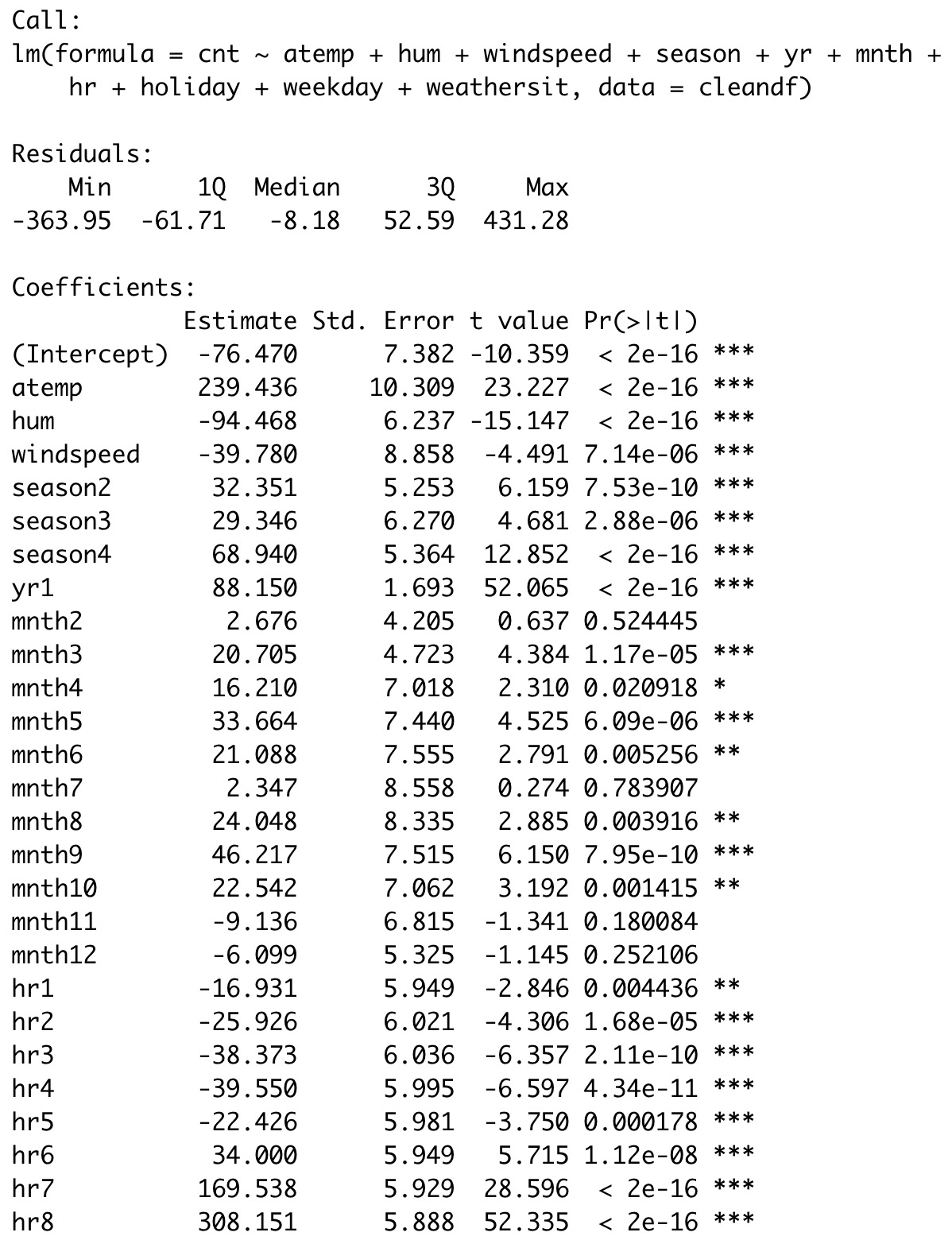
• The p-values for most of the predictor variables in the model are less than 0.05 which suggests that most of the predictor variables are statistically significant, exception being mnth2 and mnth7.
• The R-squared value of 0.6876 indicates that about 68.76% of the variance in the response variable cnt is explained by the three predictor variables atemp, hum, and windspeed.
• The adjusted R-squared value of 0.6866 is very slightly lower than the R-squared value which suggests that the model is very slightly overfit.
• The coefficient values suggest that as the temperature increases, the bike count increases. Similarly, as the humidity and windspeed increases, the bike count decreases.
• The highest coefficient for numerical variables is for atemp, suggesting that it is the most important predictor of bike count. The coefficient for atemp is 239.436, meaning that for a 1 degree increase in atemp, there is an increase in user count of 239.436 (on average).
• The highest coefficient for categorical dummy variables is for hr8 and hr17, meaning being peak hour has the greatest positive impact on user count.

Make predictions

We set the test dataset as shown, representing peak hour on a comfortable working day during the summer. We have a predicted user count of 497.585 and the 95% prediction interval of (296.0308, 699.1392).

Conclusion

The bike rental dataset contains both categorical and numerical data. After cleaning the dataset, we performed basic statistics and linear regression analysis to explore the relationship between the count of bike rentals (cnt) and various factors such as temperature (atemp), humidity (hum), and wind speed (windspeed). We found that the wind speed distribution is skewed to the right, and that the number of rental bikes increases with temperature and humidity.

Through hypothesis testing, we found factors such as hr and yr have a significant impact on the number of bike rentals.

The strength of the relationship between the count of rental bikes and the atemp, hum, and windspeed factors was determined using the coefficient of determination (R^2) value. The R^2 value for the atemp factor was 0.2, for the hum factor it was 0.1, and for the windspeed factor it was 0.0. This indicates that the relationship between the count of rental bikes and these factors is not very strong, and that there may be other factors that are more important in predicting the number of rental bikes. This is confirmed in the regression analysis.

Finally, we created a regression model with an R^2 value of 0.7. This means that the model is moderately accurate or reliable in predicting the count of rental bikes based on the factors given. Further analysis and modeling or extra variables are needed to further improve the accuracy and reliability of the prediction.

Project Members:

• Xiaoge Zhang
• Hongyi Gao