Project:Telco Customer Churn

Introduction

What is Customer Churn and Why is it Important for companies?

Customer churn is the percentage of customers that stopped using any company’s product or service during a certain time frame. We can calculate churn rate by dividing the number of customers we lost during that time period by the number of customers we had at the beginning of that time period.

For example, if the company starts the quarter with 400 customers and ends with 380, the churn rate is 5% because the company lost 5% of the total customers. Obviously, the company should aim for a churn rate that is as close to 0% as possible.

In order to achieve that, the company must know at all times what the churn rate is, and treat it as its top priority.

Telco Customer Churn Dataset

The Telco Customer Churn dataset contains information about a fictional Telco company that provides home phone and Internet services to 7043 Customers in California in Q3. It Indicates which customers have left , stayed , or signed up for their services.

As part of the final project, we are interested in finding the factors which can strongly predict the churn value for Telco. Various hypothesis tests are to be used to answer the questions and a model is to be built to predict whether the customer will be churned or not given the details related to the Customer demographics , account information and the services the Customer has signed up for.

Through our Analysis , Telco can predict the behavior to retain Customers and further develop focused Customer Retention Programs.

This data set includes information about:

• Customers who left within the last month – the column is called Churn
• Services that each customer has signed up for – phone, multiple lines, internet, online security, online backup, device protection, tech support, and streaming TV and movies
• Customer account information – how long they’ve been a customer, contract, payment method, paperless billing, monthly charges, and total charges
• Demographic info about customers – gender, age range, and if they have partners and dependents

Understanding the Dataset

This dataset was taken from the Kaggle platform and has information about the Customer data and different types of Home and Internet services they have signed up for from the Company.

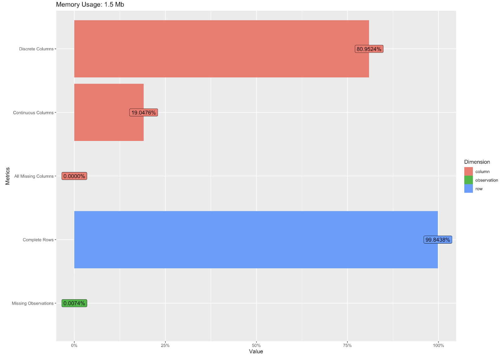
It has a total of 7043 records and 21 columns. This dataset contains both numerical and categorical types of data.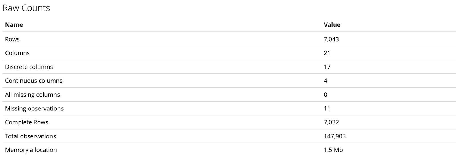

Description of the variables/features in the dataset:

Sr. No.	Feature	Dictionary
1.	Gender	The customer’s gender: Male, Female
2.	Senior Citizen	Indicates if the customer is 65 or older: Yes, No
3.	Partner	Indicates if the customer is married or not.
4.	Dependents	Indicates if the customer lives with any dependents: Yes, No.
5.	Tenure	Indicates the total amount of Tenure (In months) that the customer has been with the company by the end of the quarter
6.	Phone Service	Indicates if the customer subscribes to home phone service with the company: Yes, No
7.	Multiple Lines	Indicates if the customer subscribes to multiple telephone lines with the company: Yes, No
8.	Internet Service	Indicates if the customer subscribes to Internet service with the company: No, DSL, Fiber Optic, Cable
9.	Online Security	Indicates if the customer subscribes to an additional online security service provided by the company: Yes, No
10.	Online Backup	Indicates if the customer subscribes to an additional online backup service provided by the company: Yes, No
11.	Device Protection	Indicates if the customer subscribes to an additional device protection plan for their Internet equipment provided by the company: Yes, No
12.	Tech Support	Indicates if the customer subscribes to an additional technical support plan from the company with reduced wait times: Yes, No
13.	Streaming TV	Indicates if the customer uses their Internet service to stream television programing from a third party provider: Yes, No. The company does not charge an additional fee for this service.
14.	Streaming Movies	Indicates if the customer uses their Internet service to stream movies from a third party provider: Yes, No. The company does not charge an additional fee for this service.
15.	Contract	Indicates the customer’s current contract type: Month-to-Month, One Year, Two Year.
16.	Paperless Billing	Indicates if the customer has chosen paperless billing: Yes, No
17.	Payment Method	Indicates how the customer pays their bill: Bank Withdrawal, Credit Card, Mailed Check
18.	Monthly Charges	Indicates the customer’s current total monthly charge for all their services from the company.
19.	Total Charges	Indicates the customer’s total charges, calculated to the end of the quarter .
20.	Churn	Yes = the customer left the company this quarter. No = the customer remained with the company. Directly related to Churn Value
21.	Customer ID	A unique ID that identifies each customer.

Questions plan to answer through Analysis:

• What are the factors/services that would help predict the Customer Churn ?
• Do any of the Services that Customer has signed up for contribute to the Customer Churn ? (e.g -Online Security , Tech Support , Streaming movies etc.)
• Does demographic information of Customers (example - Gender , Senior Citizen , Dependents etc.) contribute to Customer churn rate ?
• Are Customers with less tenure more likely to be Churned ?
• Is the average total charge same across all the types of internet service?
• Are the churned customers independent of the contract type?

Methods plan to implement during Analysis:

• One Way Anova , Two –Way Anova
• Chi-Square
• Best Subset regression method
• Logistic Regression

Data Cleaning

Below is the structure of the Raw Dataset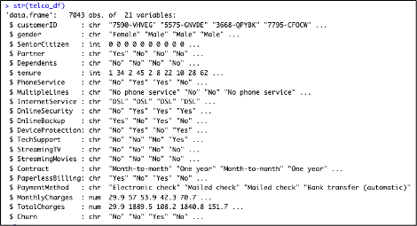

Let’s check the missing values for each attribute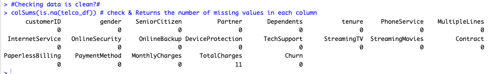

Observations:

From the above output , we can observe that there are a total 11 missing values for the TotalCharges feature. However , there is no missing value for any other attribute of the dataset.

Now , let’s handle the missing records for TotalCharges by replacing the missing values with their respective Mean and check if any missing values again in the dataframe -

Also ,As we can see from the dataset , column – Customer ID is not required or significant for our analysis , hence we would drop it .
Further , some of the features in the dataset have values - Yes & No , so we would Recode the variables - Churn , Partner , Dependents , PhoneService & PaperlessBilling to 1 & 0 respectively and make them numeric features.

Below is the structure of the final Dataset after above changes :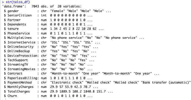

Descriptive Characteristics of the Dataset

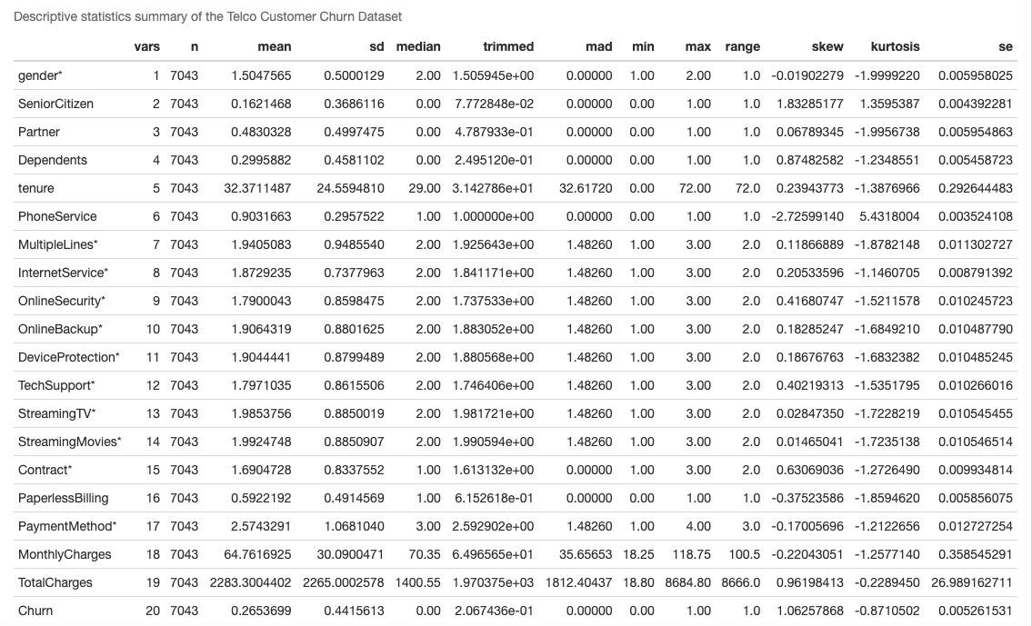
Descriptive Statistics (N, mean , median , Standard deviation, min , max , range etc.) for the entire dataset using the Describe function :

We can understand the following observations from above –

1. The mean of the Monthly Charges is $64.76, the minimum value is $18.25 and maximum is $118.75 with a standard deviation of 30.09
2. The mean of the ？Monthly Charges is $2283.30, the minimum value is $18.80 and maximum is $8684.80 with a standard deviation of 2265.
3. The mean Churn value is 0.26 with standard deviation of 0.44
4. The mean Tenure is 32.37 , the minimum value is 0 and maximum is 72 months with a standard deviation of 24.55

Correlation Plot & Check for MultiCollinearity

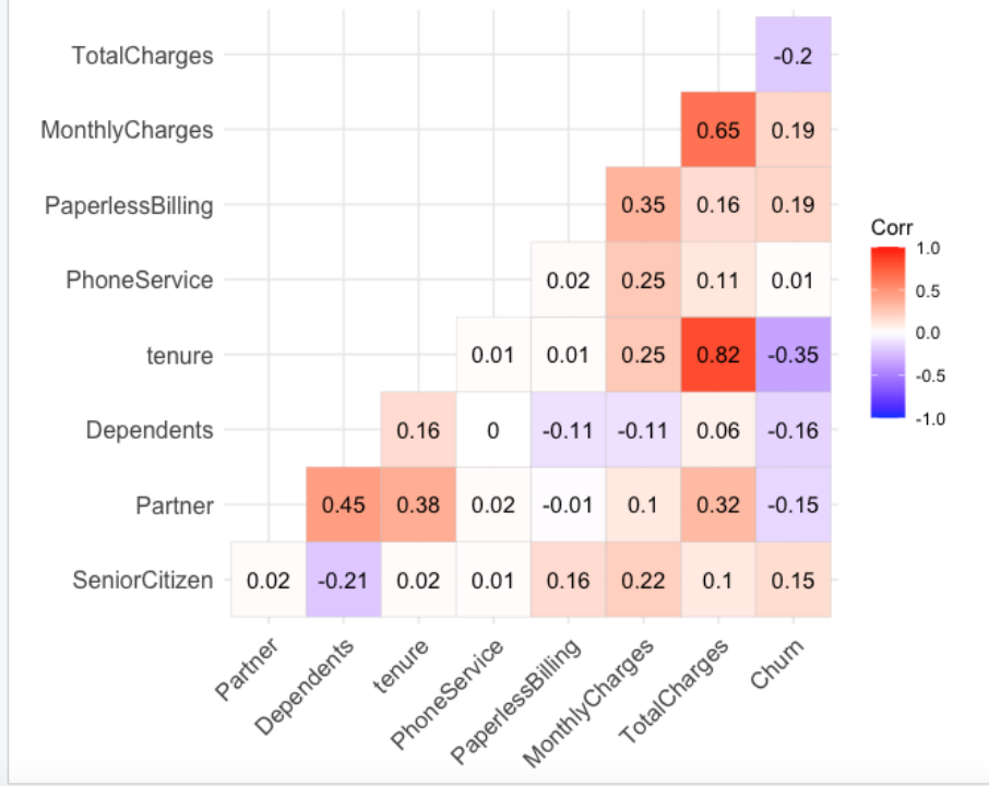
Lets understand the correlation between all the numeric features of this dataset with the help of correlation plot & Matrix

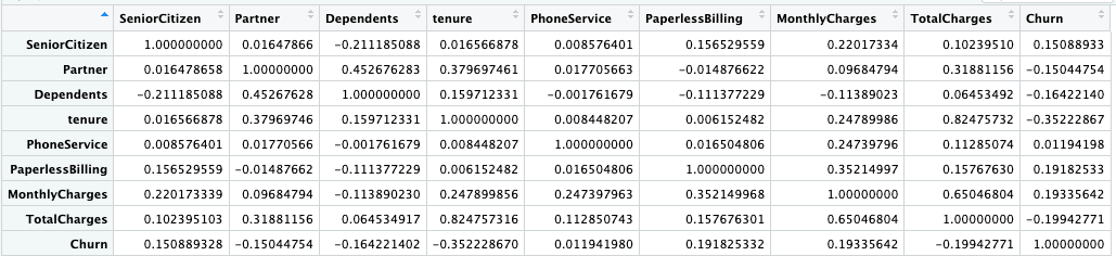
Correlation Matrix

Observations:

1. From the above Correlation plot & Matrix , we can observe that the Target Variable – Churn is positively correlated with variables – Monthly Charges with 0.193 correlation value followed by Paperless Billing with value 0.191
2. The target variable - Churn is negatively correlated with feature - Tenure with value of -0.35
3. Further, we can also see that the Monthly charges feature is highly correlated with the Total Charges with 0.65 correlation value.
4. Also , Tenure feature is highly correlated with the Total Charges with 0.82 correlation value.

Exploratory Data Analysis:

1. Does the gender attribute of a customer have an impact on the customer churn?

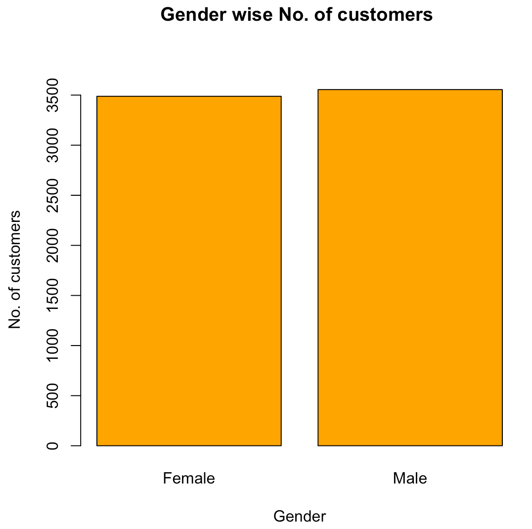
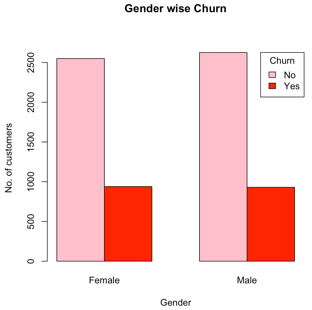
From the above graphs, we are able to infer that the churn rate is the same for both male and female customers and there is no impact of gender found in the churn rate.

2. Do senior citizens have more likelihood to churn?

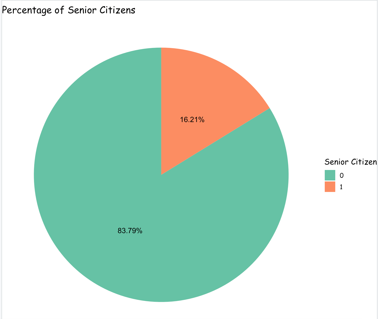
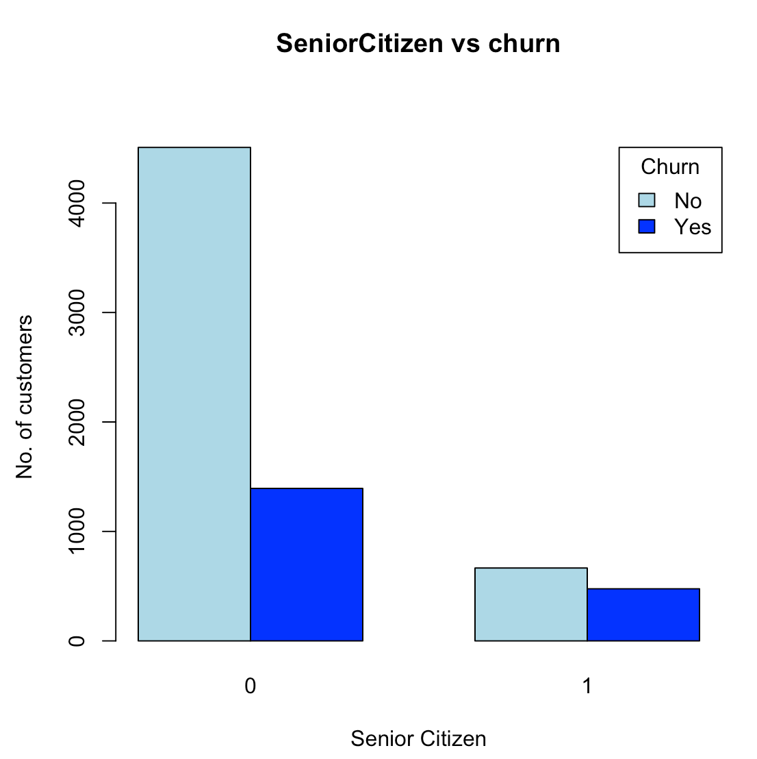
From the above graphs, it can be observed that there are a very less number of senior citizens signed up as a customer than the young/middle aged people. With respect to customer churn rate, the percentage of senior citizens churned is greater than the percentage of young/middle aged people.

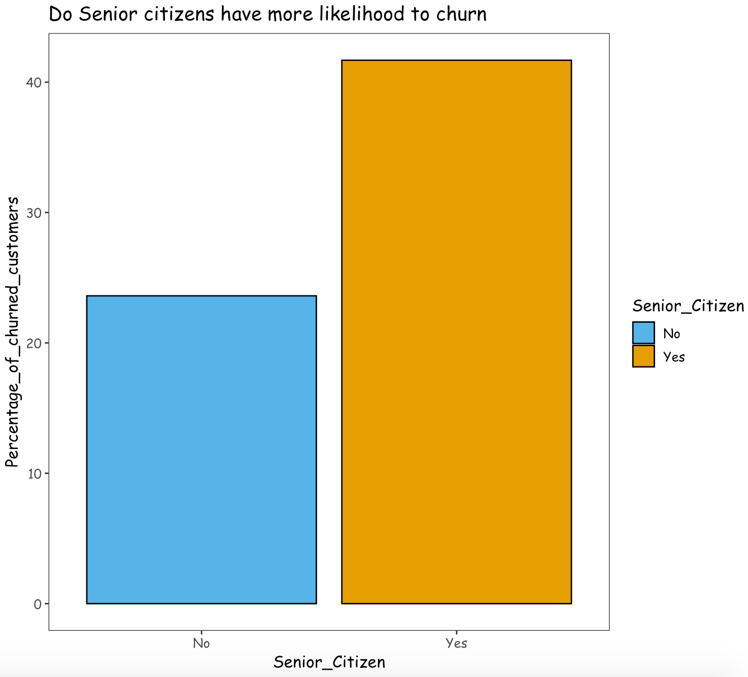
Thus, it can be inferred that the company is only able to retain around 60% of the Senior citizens and the remaining 40% of the Senior citizens have left the company. Compared to young/middle aged people, senior citizens have more likelihood to churn.

3. Are the customers having a longer tenure with the company less likely to churn?

   

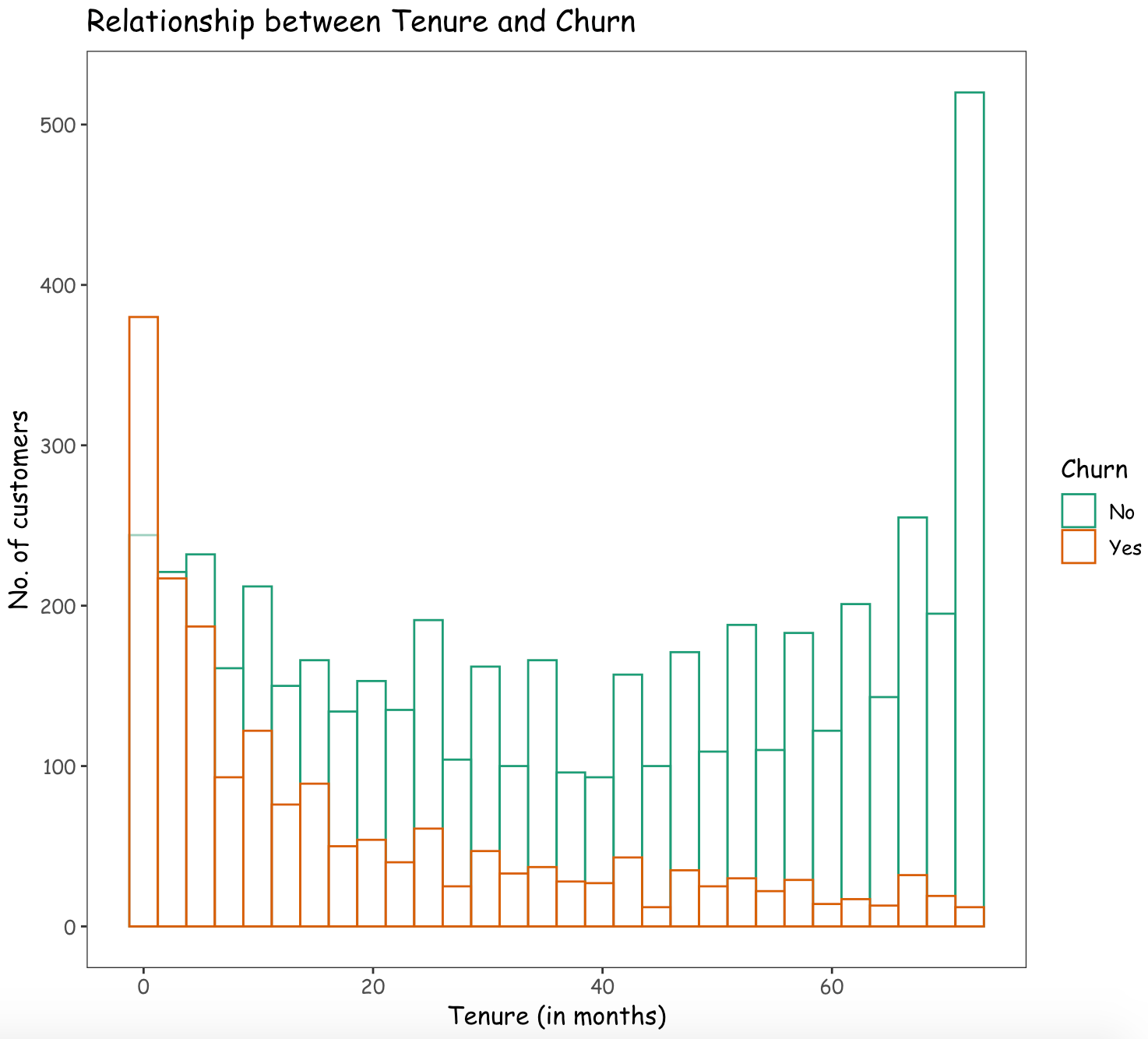
From the above graph, it can be inferred that as a customer has a longer tenure with the company, there is a reduction in the likelihood to churn.

4. Which contract type has the most number of churns?

   

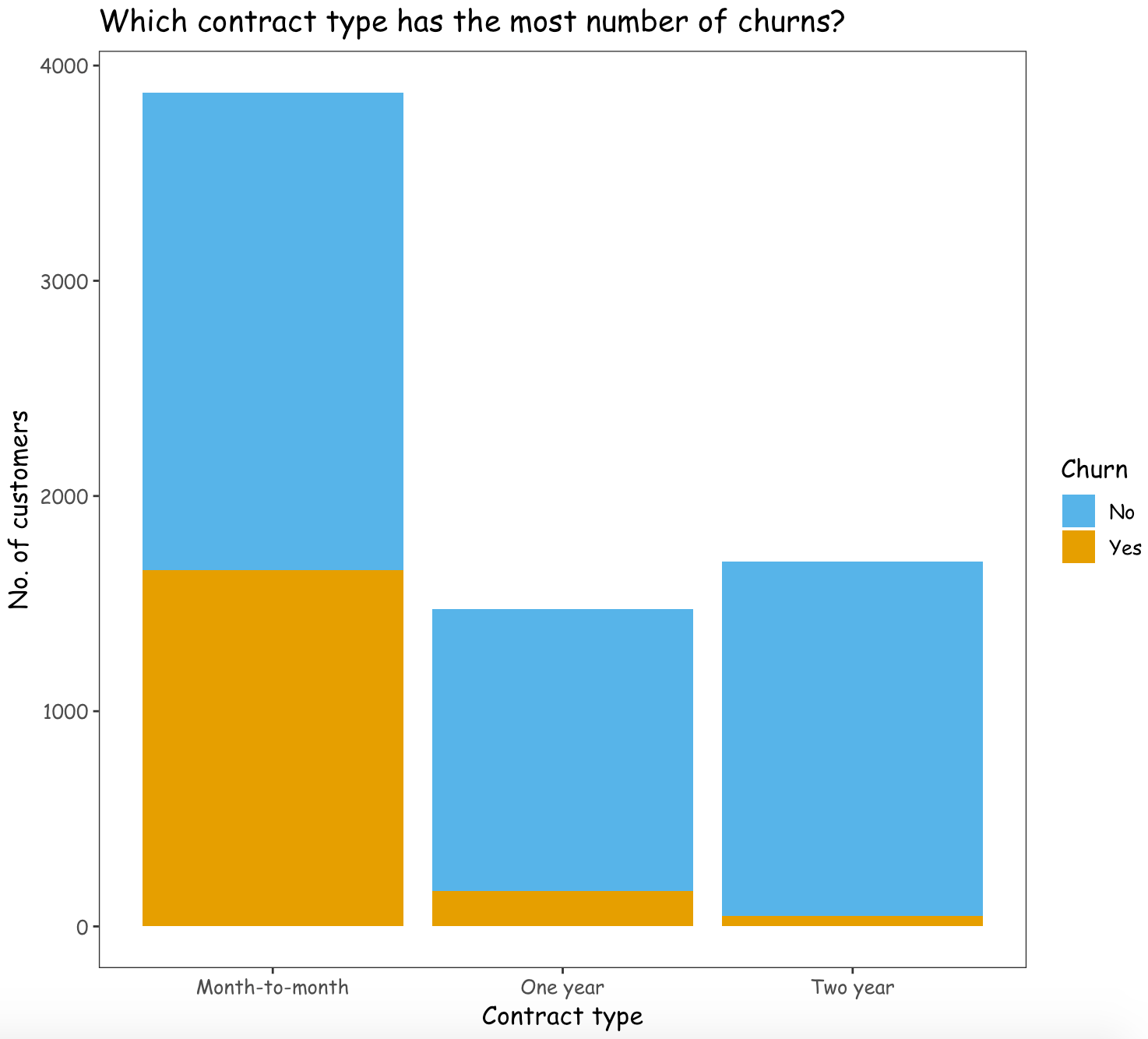
The customers with a contract type of Month-to-month are more likely to churn than the customers with other contract types.

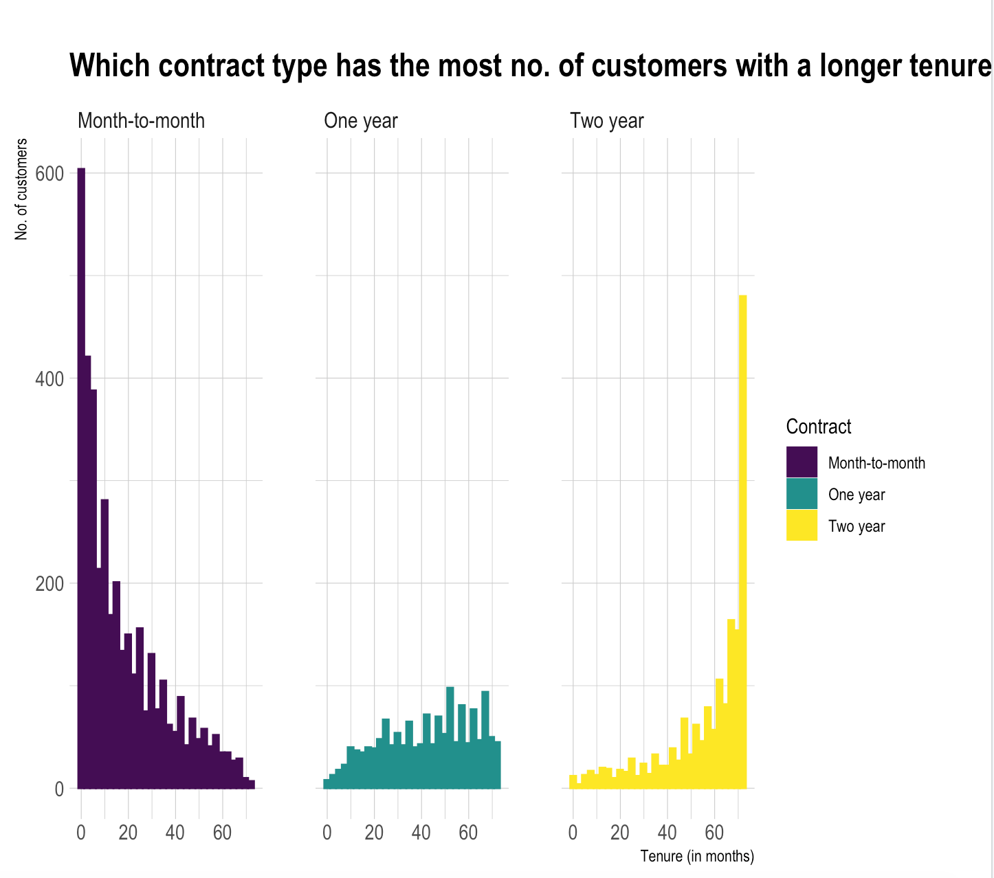
The number of customers having a Two-year contract type with a longer tenure period are comparatively greater and hence two-year contract type can result in lesser number of customers getting churned.

The number of customers having a Month-to-month contract type with a longer tenure period are comparatively lesser and hence Month-to-month contract type can result in more number of customers getting churned.

5. Which Internet service contributes to the maximum number of churned customers?

   

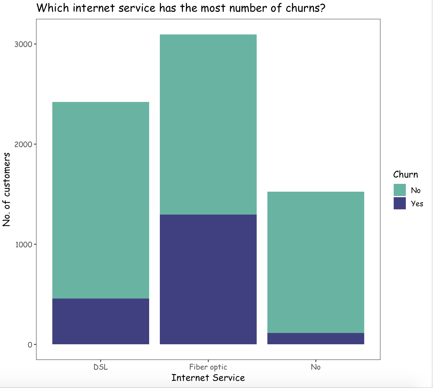
From the above graph, it can be observed that the customers opting for an internet service type of Fiber optic, are more likely to churn than with other internet services.

Methods - Chi Square (test of independence)

1. Are the churned customers independent of the contract type?

（1）State the hypotheses
Null Hypothesis: No. of churned customers are independent of the contract type attribute.
Alternate Hypothesis: No. of churned customers are dependent on the contract type attribute.

（2）Set significance level

alpha <- 0.05

（3）Create table
Creating a table to get the number of customers for each contract type and churn attribute.

（4）Compute the test value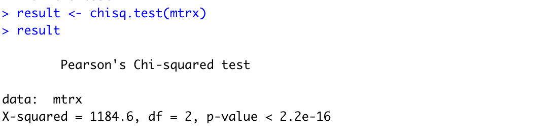

（5）Summarize the results
Conclusion : The p-value is lesser than the significance level 0.05, thus we can reject the null hypothesis and conclude that the number of churned customers are dependent on the contract type attribute.

2. Churn & PhoneService

（1）State the hypotheses
H0: There is no relationship between PhoneService and churn
H1: There is a relationship between PhoneService and churn
(significant level of 0.05)

（2）Set significance level

alpha <- 0.05

（3）Compute the test value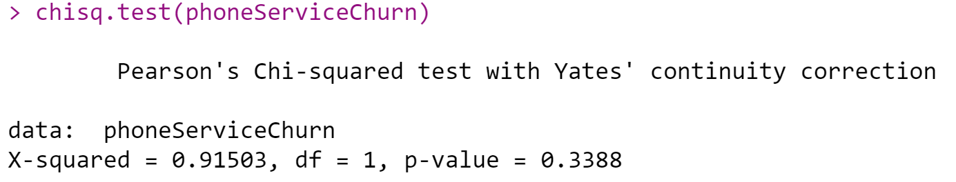

（4）Summarize the results
Since the p-value (0.3388) is greater than the significance level of 0.05, we do not reject H0. There is not sufficient evidence that supports there is a relationship between PhoneService and churn.

3. Churn & Gender

（1）State the hypotheses
H0: There is no relationship between gender and churn
H1: There is a relationship between gender and churn
(significant level of 0.05)

（2）Set significance level

alpha <- 0.05

（3）Compute the test value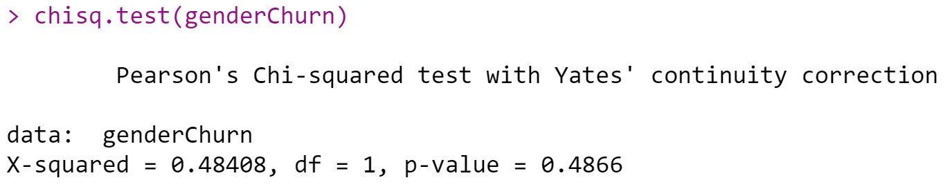

（4）Summarize the results
Since the p-value (0.4866) is greater than the significance level of 0.05, we do not reject H0. There is not sufficient evidence that supports there is a relationship between gender and churn.

4. Churn & Partner
   （1）State the hypotheses
   H0: There is no relationship between partner and churn
   H1: There is a relationship between partner and churn

（2）Set significance level

alpha <- 0.05

（3）Compute the test value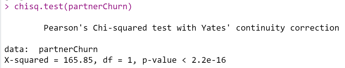

（4）Summarize the results
Since the p-value (0.000) is less than the significance level of 0.05, we reject H0. There is sufficient evidence that supports there is a relationship between partner and churn.

5. Churn & Tenure
   （1）State the hypotheses
   H0: There is no difference in the duration of tenure.
   H1: There is a difference in the duration of tenure.

（2）Set significance level

alpha <- 0.05

（3）Compute the test value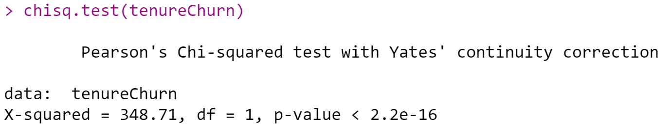

（4）Summarize the results
Since the p-value (0.000) is less than the significance level of 0.05, we reject H0. There is a difference in the duration of tenure. The duration of tenure is less than the mean that the customer churn is 38%, and the duration of tenure is more than the mean that the customer churn is 18.1%. So Customers with less tenure are more likely to be Churned.

One-way ANOVA

1. Is the average total charge same across all the types of internet service?

（1）State the hypotheses
Null Hypothesis: The mean total charge is the same for all types of internet service.
Alternate Hypothesis: The mean total charge is different for all types of internet service.

（2）Set significance level

alpha <- 0.05

（3）Create data frame

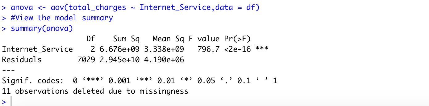
Forming a data frame to hold the total chargers for each type of internet service.

dsl <- sqldf("select * from telco_df where InternetService = 'DSL'")

fo <- sqldf("select * from telco_df where InternetService = 'Fiber optic'")

no <- sqldf("select * from telco_df where InternetService = 'No'")

dsl_df <- data.frame('total_charges' = dsl$TotalCharges,
                     'Internet_Service' = rep('DSL',nrow(dsl)),
                     stringsAsFactors = FALSE)

fo_df <- data.frame('total_charges' = fo$TotalCharges,
                    'Internet_Service' = rep('Fiber optic',nrow(fo)),
                    stringsAsFactors = FALSE)

no_df <- data.frame('total_charges' = no$TotalCharges,
                    'Internet_Service' = rep('No',nrow(no)),
                    stringsAsFactors = FALSE)
# Combine the dataframes into one
df <- rbind(dsl_df, fo_df, no_df)
df$Internet_Service <- as.factor(df$Internet_Service)

（4）Compute the test value
Running the one-way ANOVA test using aov() function: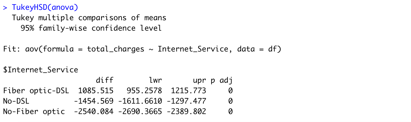

（5）Summarize the results
The p-value is lesser than the significance level 0.05, thus we can reject the null hypothesis and conclude that the average total charge is different for all types of internet service.

Tukey test can be used to identify the pair of internet services which have a significantly different mean.

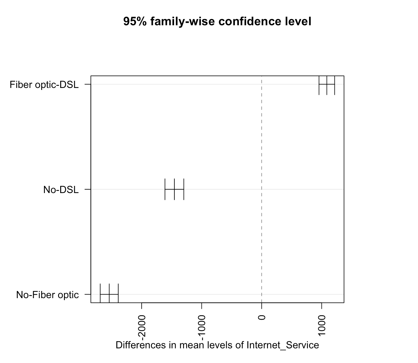
From the above graph, we are able to observe that Fiber optic - DSL internet service pair has a significant mean difference than the remaining pairs.

2. Is the mean total charges for each contract type the same?

（1）State the hypotheses
Null Hypothesis: The mean total charges for each contract type are the same.
Alternate Hypothesis: The mean total charges for at least one contract type is different.

（2）Set significance level

alpha <- 0.05

（3）Create data frame
Forming a data frame to hold the total chargers for each type of contract.

month_to_month <- telco_df[telco_df$Contract == 'Month-to-month', ]
one_year <- telco_df[telco_df$Contract == 'One year', ]
two_year <- telco_df[telco_df$Contract == 'Two year', ]

month_to_month_df <- data.frame('total_charges' = month_to_month$TotalCharges,
                                'Contract' = rep('Month-to-month', nrow(month_to_month)),
                                stringsAsFactors = FALSE)

one_year_df <- data.frame('total_charges' = one_year$TotalCharges,
                          'Contract' = rep('One year', nrow(one_year)),
                          stringsAsFactors = FALSE)

two_year_df <- data.frame('total_charges' = two_year$TotalCharges,
                          'Contract' = rep('Two year', nrow(two_year)),
                          stringsAsFactors = FALSE)

# Combine the dataframes into one
df <- rbind(month_to_month_df, one_year_df, two_year_df)

df$Contract <- as.factor(df$Contract)

（4）Compute the test value
Running the one-way ANOVA test using aov() function: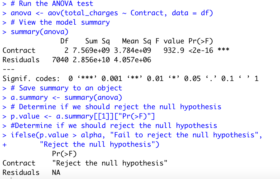

（5）Summarize the results
The p-value is lesser than the significance level 0.05, thus we can reject the null hypothesis and conclude that the average total charge is different for all types of contract.

3. Is the mean total charges for each PaymentMethod are the same?

（1）State the hypotheses
Null Hypothesis: There is no difference in the mean Total Charges for different Payment Methods.
Alternate Hypothesis: There is a difference in the mean Total Charges for different Payment Methods.

（2）Set significance level

alpha <- 0.05

（3）Create data frame
Forming a data frame to hold the total chargers for each type of contract.

electronic_check <- telco_df[telco_df$PaymentMethod == 'Electronic check', ]
mailed_check <- telco_df[telco_df$PaymentMethod == 'Mailed check', ]
bank_transfer <- telco_df[telco_df$PaymentMethod == 'Bank transfer (automatic)', ]
credit_card <- telco_df[telco_df$PaymentMethod == 'Credit card (automatic)', ]

electronic_check_df <- data.frame('total_charges' = electronic_check$TotalCharges,
                                  'PaymentMethod' = rep('Electronic check', nrow(electronic_check)),
                                  stringsAsFactors = FALSE)

mailed_check_df <- data.frame('total_charges' = mailed_check$TotalCharges,
                              'PaymentMethod' = rep('Mailed check', nrow(mailed_check)),
                              stringsAsFactors = FALSE)

bank_transfer_df <- data.frame('total_charges' = bank_transfer$TotalCharges,
                               'PaymentMethod' = rep('Bank transfer (automatic)', nrow(bank_transfer)),
                               stringsAsFactors = FALSE)

credit_card_df <- data.frame('total_charges' = credit_card$TotalCharges,
                             'PaymentMethod' = rep('Credit card (automatic)', nrow(credit_card)),
                             stringsAsFactors = FALSE)

# Combine the dataframes into one
df <- rbind(electronic_check_df, mailed_check_df, bank_transfer_df, credit_card_df)

df$PaymentMethod <- as.factor(df$PaymentMethod)

（4）Compute the test value
Running the one-way ANOVA test using aov() function: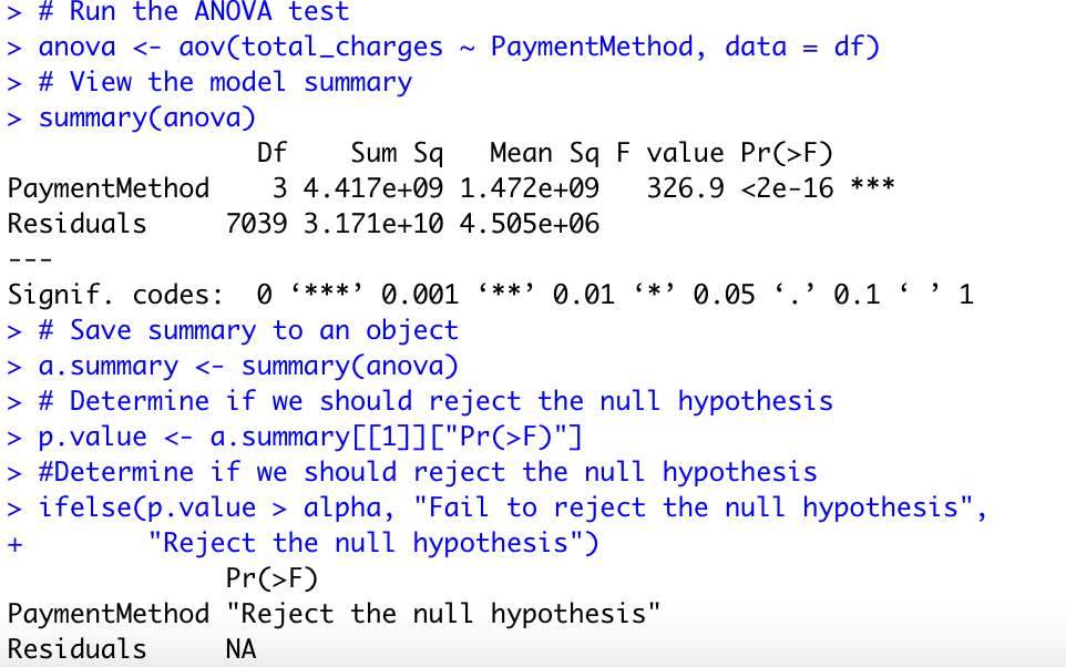

（5）Summarize the results
The p-value is lesser than the significance level 0.05, thus we can reject the null hypothesis and conclude that the average total charge is different for all types of Payment Methods.

Two-way ANOVA test

Churn & SeniorCitizen, Dependents

（1）State the hypotheses
Dependent variable: churn
Independent variables: SeniorCitizen and Dependents

H0: SeniorCitizen and Dependents have no impact on churn
H1: SeniorCitizen and Dependents have an impact on churn

（2）Set significance level
alpha <- 0.05

（3）Compute the test value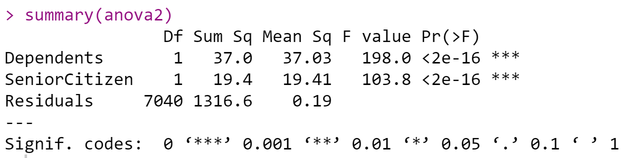

（4）Summarize the results
Since the p-value dependents (<0.0000) are less than the significance level of 0.05, and the p-value senior citizen (<0.000) is less than the significance level of 0.05, we reject H0. There is sufficient evidence that supports SeniorCitizen and Dependents have an impact on churn.

In conclusion, demographic information of SeniorCitizen, Dependents, and Partners will affect customers’ churn rate. Gender has no relationship with churn.

Splitting the data into a train and test set

To separate the data into train and test set to a 70/30 split where 70% of the random observations are used for the training set and 30% is used for testing, I have used the createDataPartition() function from the ‘caret’ package

#Split the dataset into Test and Train data#
set.seed(123)
trainIndex <- createDataPartition(telco_df$Churn, p = 0.70, list = FALSE , times=1 )
telco_df_train <- telco_df[trainIndex,]
telco_df_test <- telco_df[-trainIndex,]

#Define the Target variable for Train and Test Data set
y_train <- telco_df_train$Churn
y_test<- telco_df_test$Churn

Subset Regression Method

This method helps in the model selection process which tests all the possible combinations of the independent/explanatory variables and eventually helps in identifying the best possible Model using the regsubsets function from the leaps package.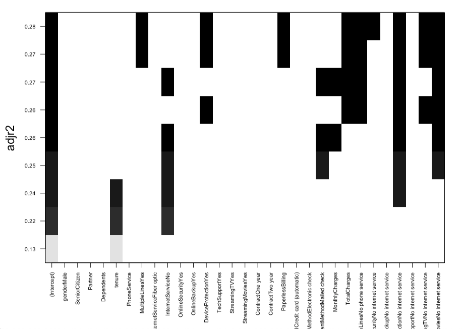

Observation: The above plot function shows the attributes from the subset Regression method that can be selected for the best Model and are ranked as per their adjusted R-square value.

Below are the Final 9 predictors identified using the Subset Regression Method-

• MultipleLines-No
• OnlineSecurity-Yes
• TechSupport-Yes
• Contract- One year, Two Year
• PaperlessBilling
• PaymentMethod- Electronic
• MonthlyCharges
• Total Charges

Let us build the models using different algorithms using Glm Logistic regression, Stepwise selection, Ridge, Lasso for predicting the customer churn and select the best model by comparing various metrics like AIC, BIC, RMSE etc.,

Logistic Regression Model Using GLM

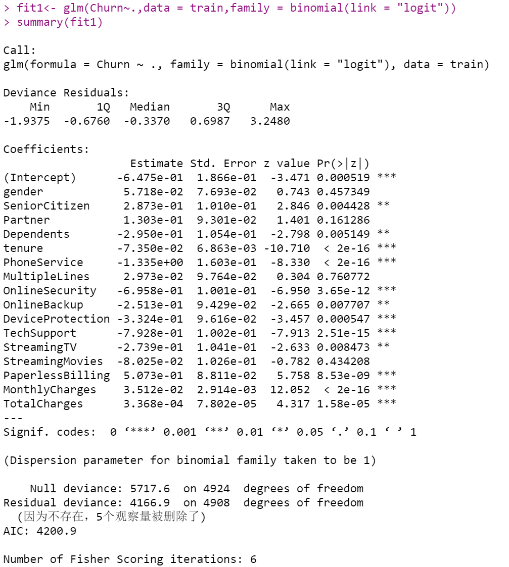
In the logistic regression model, I first used all the variables to create the model. According to the summary of the model, tenure, PhoneService, OnlineSecurity, DeviceProtection, TechSupport, PaperlessBilling, MonthlyCharges, TotalCharges, SeniorCitizen are significant variables. So in the next step, I will choose these variables to build a new model.

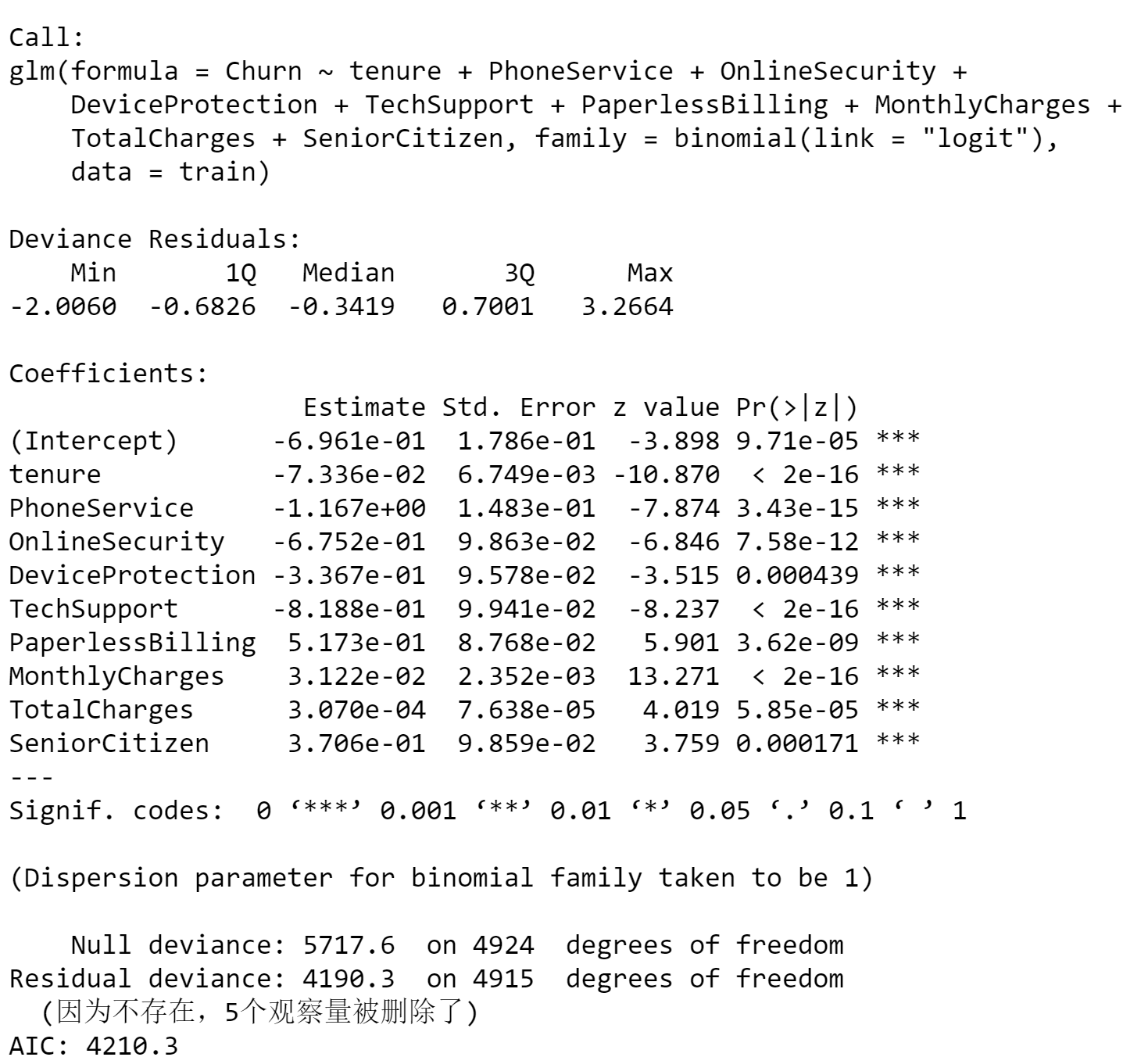
From the summary of the new model, I can see all the variables are significant now, and this is maybe a better model. In the following steps, I will use a confusion matrix to calculate the accuracy of the model.Use the confusion matrix to see if the model is a good one.

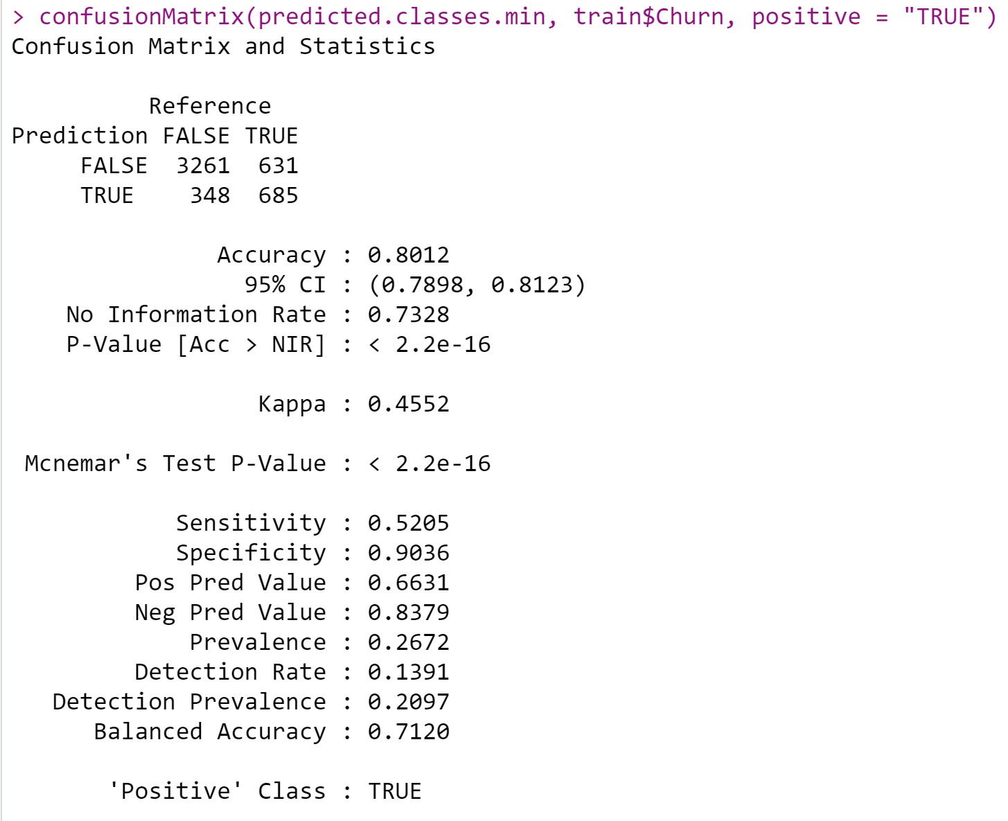
By looking at the confusion matrix, I observed an accuracy of 80.12% for this model.I don’t think this number is that high, so I want to try to improve the accuracy of the model by removing outliers.

Outliers Identification & Removal

#replace outliers with mean (tenure, MonthlyCharges,TotalCharges)
high <- mean(telco_df$tenure) + sd(telco_df$tenure) * 3
low <- mean(telco_df$tenure) - sd(telco_df$tenure) * 3
telco_df$Outlier <- (telco_df$tenure < low | telco_df$tenure > high)
telco_df$tenure[telco_df$outlier] = mean(telco_df$tenure[!is.na(telco_df$outlier)])

high <- mean(telco_df$MonthlyCharges) + sd(telco_df$MonthlyCharges) * 3
low <- mean(telco_df$MonthlyCharges) - sd(telco_df$MonthlyCharges) * 3
telco_df$Outlier <- (telco_df$MonthlyCharges < low | telco_df$MonthlyCharges > high)
telco_df$MonthlyCharges[telco_df$outlier] = mean(telco_df$MonthlyCharges[!is.na(telco_df$outlier)])

high <- mean(telco_df$TotalCharges) + sd(telco_df$TotalCharges) * 3
low <- mean(telco_df$TotalCharges) - sd(telco_df$TotalCharges) * 3
telco_df$Outlier <- (telco_df$TotalCharges < low | telco_df$TotalCharges > high)
telco_df$TotalCharges[telco_df$outlier] = mean(telco_df$TotalCharges[!is.na(telco_df$outlier)])

Since the other variables except tenure, monthlycharges and totalcharges are Categorical variables, we will replace the outliers of the three non-categorical variables with the average of all the outliers. Then I will use the new cleaning data to build the model.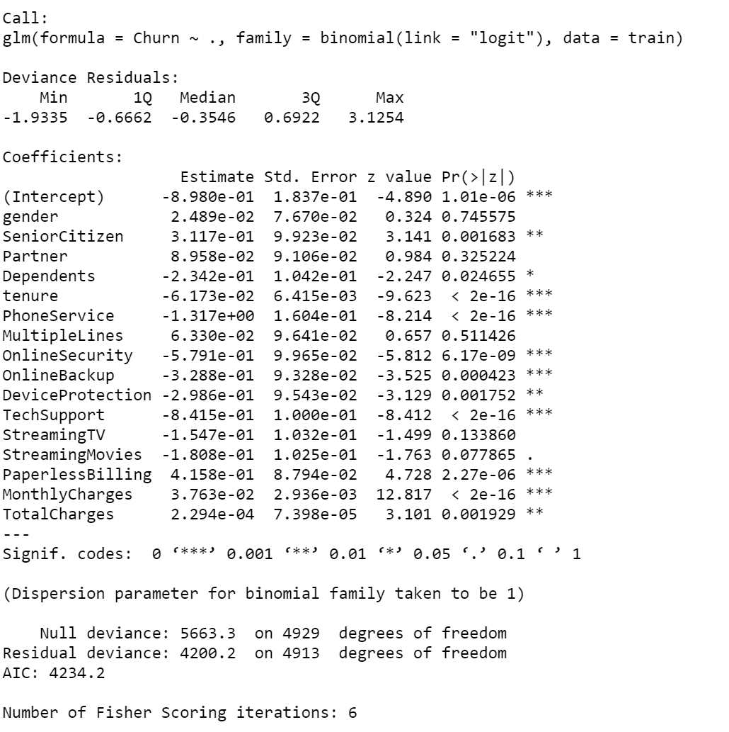

Same step here, first used all the variables to create the model. According to the summary of the model, picked up all the significant variables to built a new model.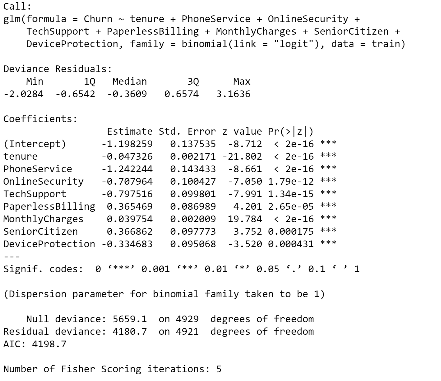

From the summary of the new model, I can see all variables are significant now, and this is maybe a better model. In the AIC measure, if the score is lower than the other one, it means this model is the preferred model. But it didn’t improve too much if we look at the AIC measure, the model 2’s AIC is a little bigger than model 1’s. However, the parameter in Model 2 is less, which is better than Model 1.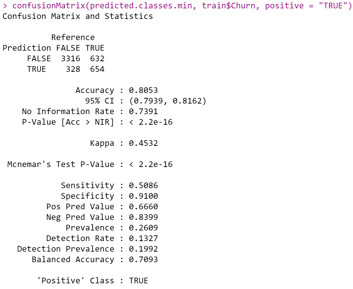

By looking at the confusion matrix, the prediction is the row and the actual value is the column.

• Accuracy: By looking at the confusion matrix figure, the accuracy is 0.8053 (80.53%), this is better than the previous model.
• Precision: Precision refers to the positive predictive value. As can be seen from the figure, the pos pred value is 0.6660 (66.6%). This indicates that 66.6% of the customers are predicted to be churned from the telco company.
• Recall: Recall refers to sensitivity. As can be seen from the figure, the sensitivity value is 0.5086 (50.86%).
• Specificity: means the proportion of customer churn correctly identified by the measurement was 91%.

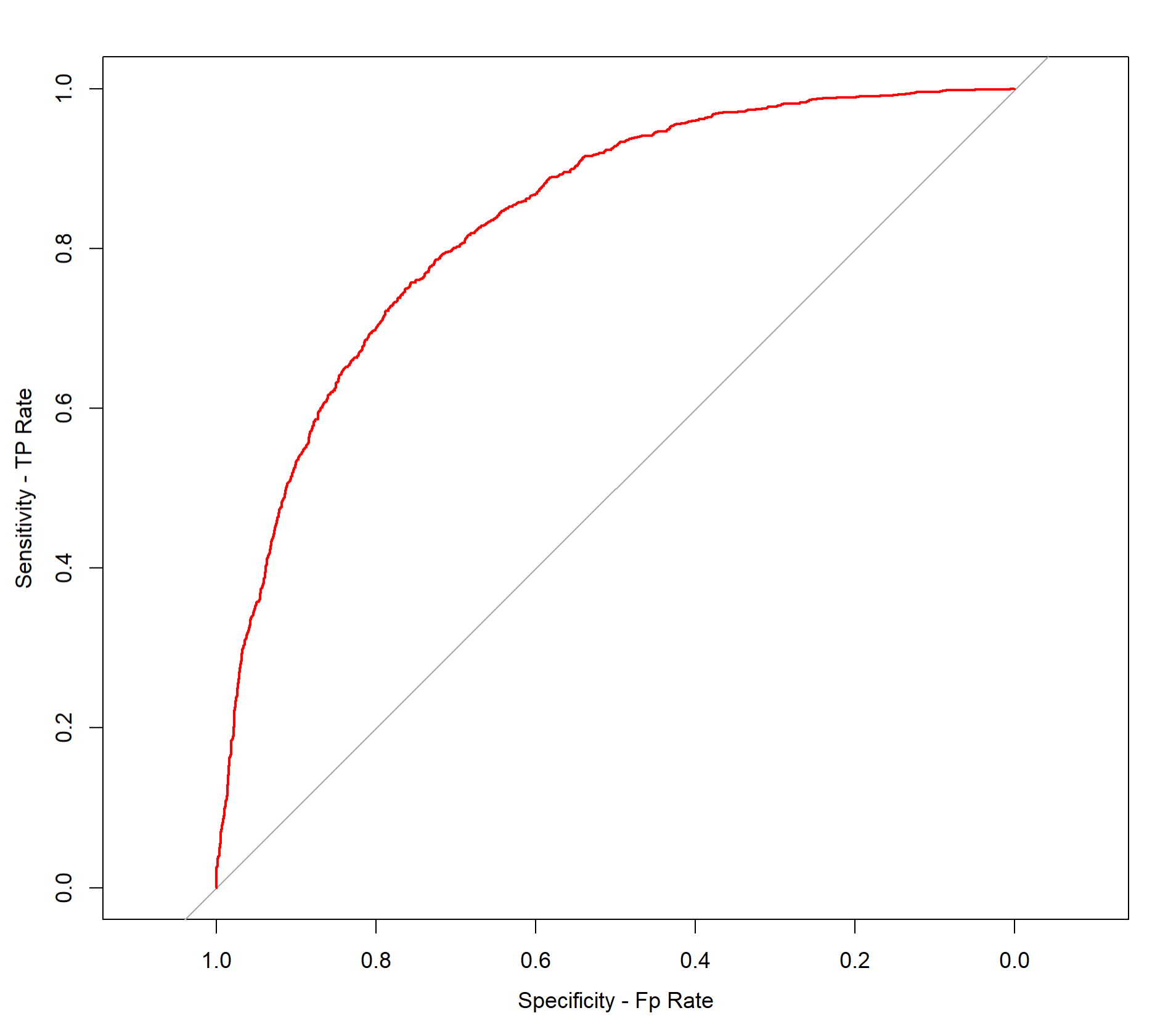
The closer the curve is to the left and upper boundaries, the more accurate the test will be. In the example of this data set, the curve is in a medium to upper state, indicating that the model is good.

Stepwise Selection

Forward selection

fullModel = lm(Churn ~ ., data = telco_test) # model with all variables
nullModel = lm(Churn ~ 1, data = telco_test) # model with the intercept only

The full model contains all variables in the dataset and the null model only has an intercept.

summary(stepAIC(nullModel, # start with a model containing no variables
                direction = 'forward', # run forward selection
                scope = list(upper = fullModel, # the maximum to consider is a model with all variables
                             lower = nullModel), # the minimum to consider is a model with no variables
                trace = 0)) # do not show the step-by-step process of model selection

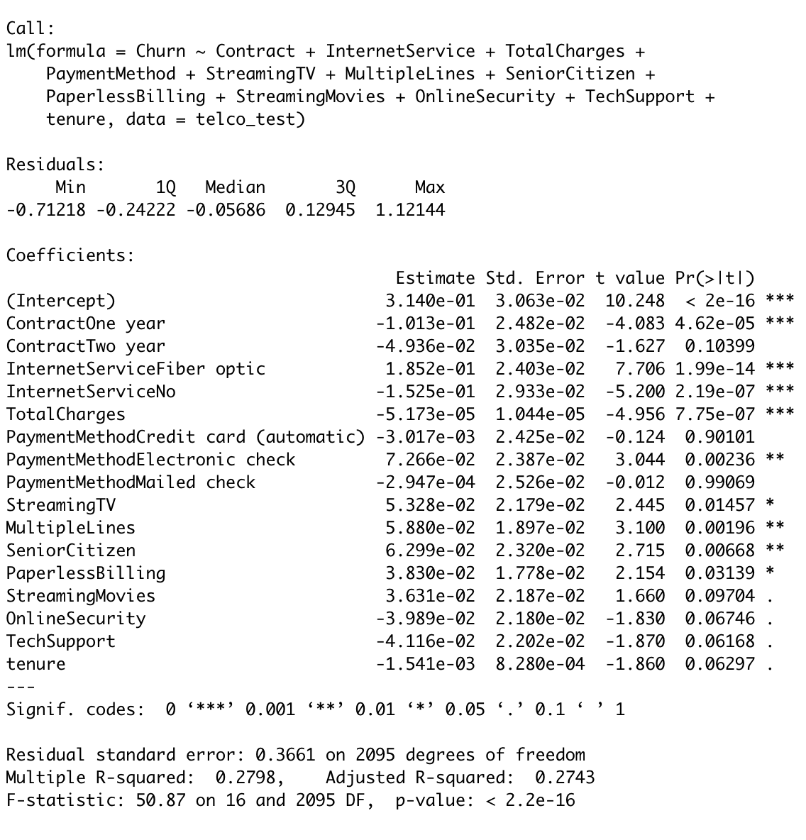
After running the stepwise forward selection, the final model selected by the AIC criterion includes the following predictors: Contract type (one year or two year), Internet service type (fiber optic or not), Total charges, payment method (electronic check), streaming TV, multiple lines, senior citizen, paperless billing, streaming movies, online security, tech support, and tenure.

• The residual standard error is 0.3661, which is a measure of the variability of the residuals.
• The multiple R-squared value of 0.2798 indicates that the model explains 27.98% of the variability in the response variable
• The adjusted R-squared value of 0.2743 indicates that the model accounts for 27.43% of the variability after adjusting for the number of predictors in the model.
• The F-statistic of 50.87 with a p-value of <2.2e-16 indicates that the model as a whole is a good fit to the data.

Calculating the AIC and BIC metrics:

stepAIC = stepAIC(nullModel, direction = 'forward',
                  scope = list(upper = fullModel, lower = nullModel),
                  trace = 0)

The AIC value of 1768.383 and BIC value of 1870.18.

Calculating the ROC and AUC scores:

model <- lm(Churn ~ ., data = telco_test)
predictions <- predict(model, type = "response")
predictions <- predict(fullModel, type = "response")
roc_object <- roc(telco_test$Churn, predictions)
auc(roc_object) # calculate the AUC score
plot(roc_object)

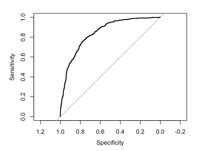
The AUC score of 0.8439 indicates that the model has a good level of accuracy in predicting the binary outcome variable. A score of 0.8439 suggests that the model has a relatively high level of accuracy in predicting the outcome variable.

Calculating RMSE:

rmse(telco_test$Churn, predict(stepAIC , telco_test))
rmse(telco_train$Churn, predict(stepAIC , telco_train))

LASSO REGRESSION

Estimating the Lambda Value using Cross Validation for Lasso Regression

The best value of Lambda is calculated using the cv.glmnet function ,alpha=1 and family = binomial as the response type for computing the penalized Lasso Regression Model using the Training set of target and predictor variables as shown below :

#Perform k-fold cross-validation to find optimal lambda value for Lasso #
set.seed(123)
lasso_cv <- cv.glmnet(x_train, y_train, family="binomial", alpha=1,nfolds = 10)
lasso_cv

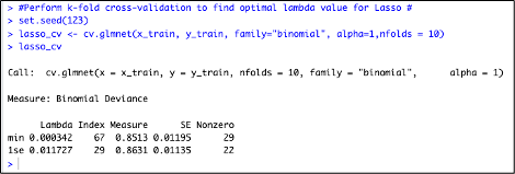
Observation : The minimum value of Lambda is 0.000342 and the value of Lambda at One Standard error is 0.011727

Below is the Logarithmic value of Lambda minimum and Lambda at One Standard Error –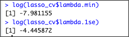

Now , lets plot Binomial Deviance and Log Lamba value as show below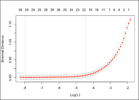

Observation: The above plot displays the cross validation error according to the log of Lambda
1.The left-dashed vertical line indicates that the log of optimal value of Lambda which is approx. -8 and is the one which minimizes the prediction error.
2.The log of lambda value at one standard error is approx -4.5

Lasso Regression Model with Training Data:

1.Below is the Lasso regression model using the glmnet function on the training data using the Minimum Lambda Value :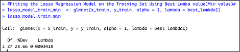

Lets , have a look at the coefficients for the above Lasso Regression Model using the Lamba Min

Observation: From the above plot coefficients of the Lasso Regression Model, we can understand the below:

1. Features with very less coefficient values have been penalized or shrunk to 0 by the Lasso Regression Model. The more they are penalized or shrunk, the less significant these features are to the model.

2. Below are the coefficients which we can understand have been shrunken to 0

• MultipleLines-No phone service
• OnlineSecurity-No internet service
• MonthlyCharges

2.Below is the Lasso regression model using the glmnet function on the training data using the Lamba Value at 1se :

Lets , have a look at the coefficients for the above Lasso Regression Model using the Lamba 1se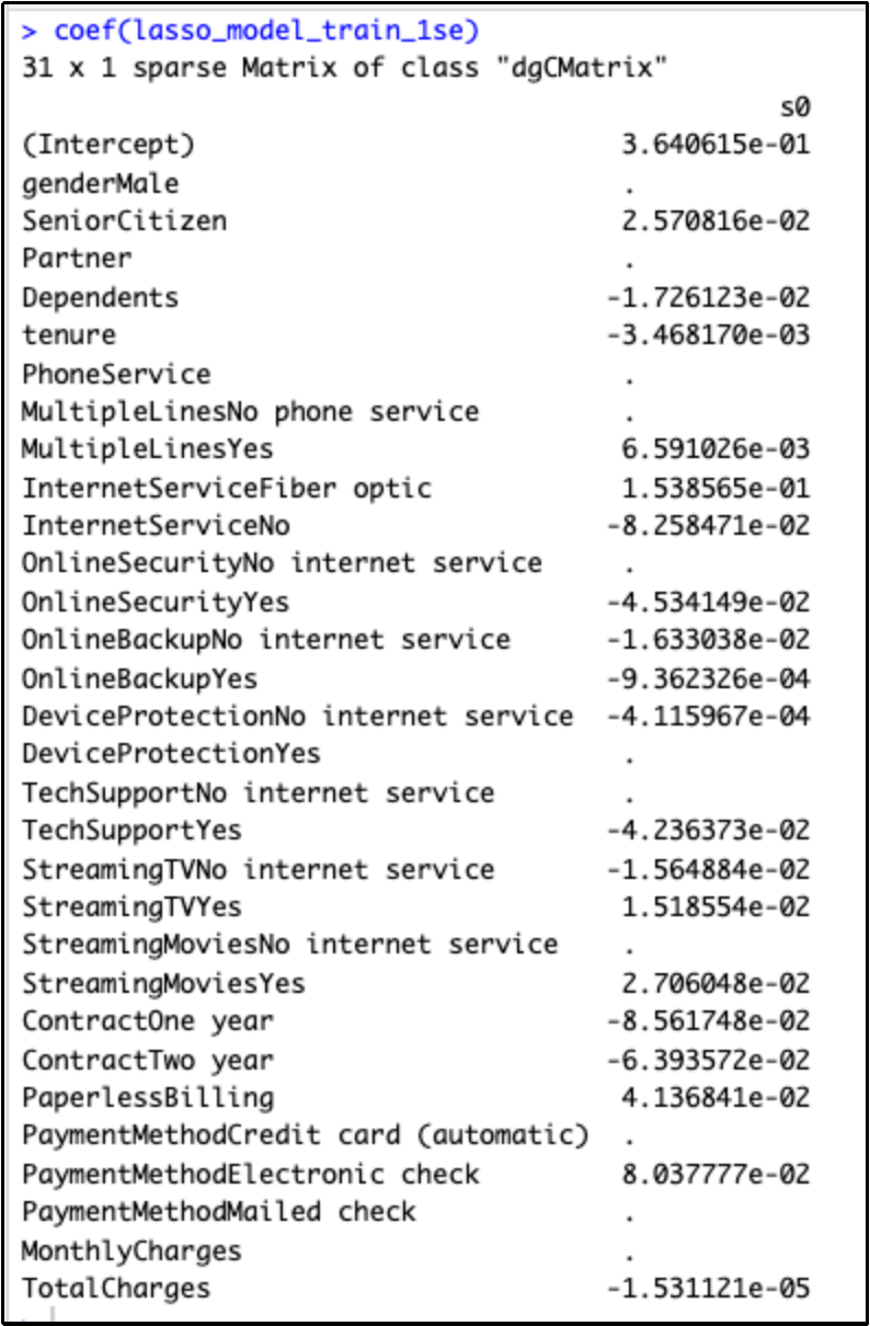

Observation: From the above plot coefficients of the Lasso Regression Model using Lambda 1se, we can understand the below:

1. Features with very less coefficient values have been penalized or shrunk to 0 by the Lasso Regression Model. The more they are penalized or shrunk, the less significant these features are to the model.
2. Below are the coefficients which we have been shrunken to 0 which are more as compared to the Model using the Lambda Min

• Gender - Male
• Partner
• Phone Service
• MultipleLines-No phone service
• OnlineSecurity-No internet service
• DeviceProtection -Yes
• TechSupport-No internet service
• StreamingMovies- No internet service
• PaymentMethod- Credit card (automatic)
• PaymentMethod-Mailed check
• MonthlyCharges

Prediction on the Training Dataset and Determining Performance of the model :

#Lasso regression model for making predictions on Train data#
predict_lasso_train <- predict(lasso_model_train_min, newx = x_train)

Root Mean Squared Error :

#RMSE for Lasso regression model against the Training set#
lasso_train_rmse <- rmse(y_train, predict_lasso_train)
lasso_train_rmse

The RMSE is 0.3768874.

Observation:

1. We first use the predict function on the Lasso Model we created using Lambda Min value to generate prediction on the training data.
2. Further , the performance of the Lasso Regression Model against the training dataset is determined by calculating the Root Mean Squared error (RMSE) using the rmse function on the predicted model.
3. Finally , we get the RMSE value on the training data which is 0.37
4. This shows that the RMSE value is good enough for the prediction as the data points in the training data are not scattered much.

Prediction on the Testing Dataset and Determining Performance of the model :

#Lasso regression model for making predictions on Test data#
predict_lasso_test <- predict(lasso_model_train_min, newx = x_test)

Root Mean Squared Error :

#RMSE for Lasso regression model against the Test set#
lasso_test_rmse <- rmse(y_test, predict_lasso_test)
lasso_test_rmse

The RMSE is 0.3768874.

Observation:

1. We first use the predict function on the Lasso Model we created using Lambda Min value to generate prediction on the training data.
2. Further , the performance of the Lasso Regression Model against the training dataset is determined by calculating the Root Mean Squared error (RMSE) using the rmse function on the predicted model.
3. Finally , we get the RMSE value on the training data which is 0.36
4. This shows that the RMSE value is good enough for the prediction as the data points in the training data are not scattered much.

Is the Model Over-fitting ?

As we saw that the RMSE values for both the Training and Test data set are almost close, hence we can conclude that the Ridge Regression Model is not over-fitting.

Lasso Model Metrics

1.AIC $ BIC Score

#AIC SCORE#
AIC.glmnet <- function(glm_fit) {
  chisqLR <- glm_fit$nulldev - deviance(glm_fit)

  chisqLR - 2*glm_fit$df
}
AIC.glmnet(lasso_model_train_min)

The AIC score is 227.3354.

#BIC SCORE#
glmnet_cv_bic(lasso_cv)

The BIC score is -1397.502.

2.The R-squared and Root Mean Square Error values (RMSE) for both Training & Test dataset is summarized as follows :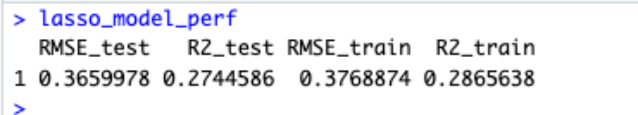

Observation :

1. R-square value for Train : 0.28
2. RMSE value for Train : 0.37
3. R-square value for Test : 0.27
4. RMSE value for Test : 0.36

ROC Curve (Receiver Operating Characteristics) and AUC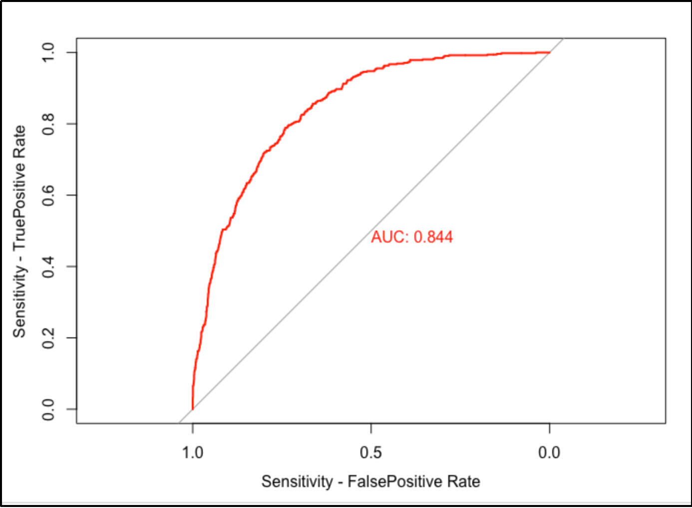

Observation :
We can observe that the ROC curve is moderately closer or hugging the y-axis and is showing a curve and is not flat at the top which indicates that the Model has shown moderate performance results.

Ridge Regression

In order to find the lambda value which produces the lowest test MSE, k-fold cross validation should be performed.

If a model is trained and tested using only one dataset, the test MSE can vary greatly depending on which observations were used in the training and testing datasets.

In order to avoid this problem, a model can be fit several times using different training and testing datasets each time and the overall test MSE can be calculated as the average of all of the test MSEs.

This method is known as cross validation and k-folds cross validation can be performed in R using cv.glmnet() function. It performs k-folds cross validation using k = 10 folds.

Alpha value of 0 should be set for Ridge regression models.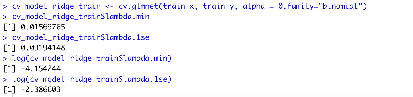

Lambda.min has a value of 0.015 and Lambda.1se has a value of 0.09.

Lambda.min gives the result with minimum mean cross-validation error. It is the lambda value at which the smallest MSE and maximum accuracy can be achieved. This lambda value will give the most accurate model.

Lambda.1se gives the result such that the cross-validation error is within 1 standard error of the minimum. This lambda value gives the simplest model and also lies within 1 standard error of the optimal value of lambda.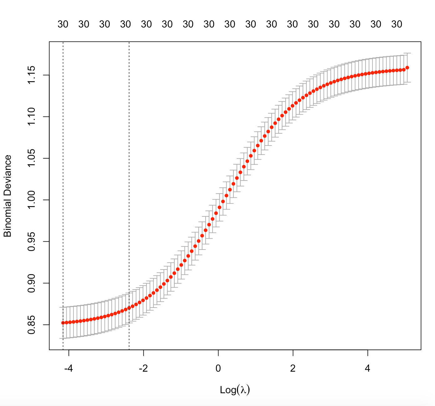

The left dashed vertical line gives the log of the optimal lambda value (Lambda.min) which produces the least prediction error , its value is approximately equal to -4.15.
The right dashed vertical line gives the log of the lambda value (Lambda.1se) which can produce the simplest model. Its value is approximately equal to -2.38.

Fitting the Ridge regression model:

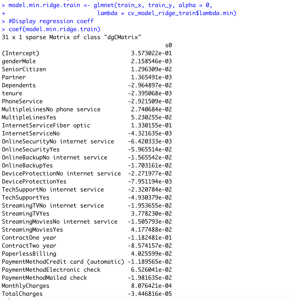
Fitting the Ridge regression model using the best lambda value which can produce the least prediction error - Lambda.min - glmnet() function is used against the training dataset and the coefficients of the predictor variables are displayed.
All the significant variables are incorporated in the model. Thus the maximum possible accuracy of the model is achieved and the prediction error is reduced by imposing a penalty to the model for having too many variables.

Making predictions for the training dataset: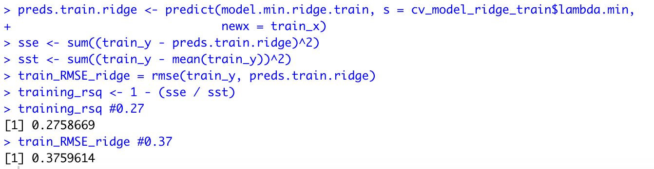

The Root mean square error value is calculated using the rmse() function of the Metrics package. The value of RMSE for this model is 0.37.
The R square value is calculated using the formula 1 - (sse/sst) and the value is 0.27.
Generally, the smaller the RMSE , the better is the model performance. The R square value for this model is quite less , with a value of 0.27 which means that 27 percent of the variance in the results is explained by the predictor variables. This model accuracy is very low and not reliable.

Making predictions for the testing dataset: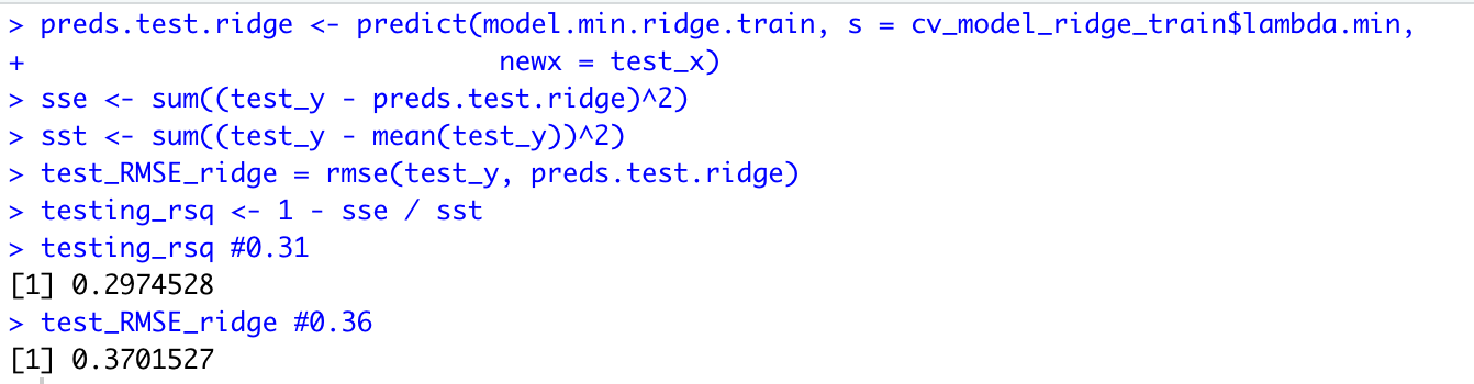

The Root mean square error value is calculated using the rmse() function of the Metrics package and the value with the testing dataset is calculated as 0.37.
The R square value is calculated using the formula 1 - (sse/sst) and the value with the testing dataset is 0.29.
We can determine if a model is overfit by calculating the difference between RMSE of the training and testing datasets.
= 0.37 - 0.37 = 0
If this difference in RMSE between the training and testing datasets is close to 0, the model is not overfit. The difference of RMSE is 0 and also the R square value is almost equal in both training dataset and testing dataset, which means that there is no problem of overfitting observed with this model.

Calculating the AIC and BIC metrics:

AIC.glmnet <- function(glm_fit) {
  chisqLR <- glm_fit$nulldev - deviance(glm_fit)

  chisqLR - 2*glm_fit$df
}

AIC.glmnet(model.min.ridge.train)

The AIC is 205.0926.

glmnet_cv_aicc <- function(fit, lambda = 'lambda.min'){
  whlm <- which(fit$lambda == fit[[lambda]])
  with(fit$glmnet.fit,
       {
         tLL <- nulldev - nulldev * (1 - dev.ratio)[whlm]
         k <- df[whlm]
         n <- nobs
         return(list('BIC' = log(n) * k - tLL))
       })
}

#AIC and BIC scores for Ridge regression
glmnet_cv_aicc(cv_model_ridge_train)

The BIC is -1185.51.

Calculating the ROC and AUC scores: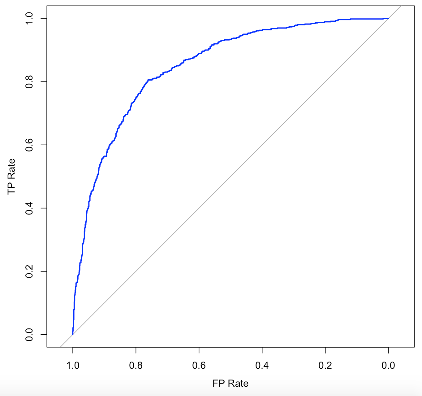

The ROC curve is approaching the central diagonal line which indicates that the model performance is moderate. The area under the curve value is 0.84. The higher the AUC, the model has good discriminatory ability and it will correctly predict the true positives and negatives for 84% of the time.

Important metrics for the model:

AIC : 205.09
BIC : -1185.51
RMSE (Training RMSE - Testing RMSE) : 0
R Square Test : 0.27
R Square Train : 0.27
AUC : 0.84

COMPARISON OF THE MODELS

METRICS	LOGISTIC MODEL - GLM	STEPWISE - Forward	LASSO	RIDGE
AIC	4198.7	1768.383	227.33	205.09
—	—	—	—	—
BIC	4257	1870.18	-1397.50	-1185.51
—	—	—	—	—
RMSE (Difference of Training & Test)	0.022	0.01	0.01	0.01
—	—	—	—	—
AUC	0.8351	0.8439	0.844	0.84
—	—	—	—	—

Observations:
The model built using the Logistic regression algorithm with Glm() function in R did a good job in predicting the customer churn with a RMSE difference value between training and testing datasets of 0.02. This means that the difference between the actual and the predicted values is very less and it performed well in both the training and testing datasets. The AUC score of this model is 0.83, indicating that this model can correctly classify the samples for 83% of the time.

AIC and BIC scores provide measures of the model performance that account for model complexity. These values are quite large and hence this model is quite complex though it can be accurate with the predictions.

In order to achieve a simpler model, we used the Stepwise selection method, Ridge and Lasso algorithms.

Used Stepwise selection algorithm (forward) to select the best set of predictor variables : Contract type (one year or two year), Internet service type (fiber optic or not), Total charges, payment method (electronic check), streaming TV, multiple lines, senior citizen, paperless billing, streaming movies. A comparatively lower AIC and BIC scores were achieved.

Ridge and Lasso regularization algorithms were used to build models to check if the complexity of the model can be reduced further. Both Lasso and Ridge models had a very low RMSE in both training and testing datasets and were able to predict the results accurately for 84% of the time.

All the above models achieved almost the same level of accuracy.

In general, BIC is more conservative than AIC and tends to select simpler models, while AIC is more flexible and may select models with a higher complexity.

As we are trying to reduce the complexity of the model, we can select the Lasso regression model as the best model as it has the lowest BIC value.

CONCLUSION

In this project , a dataset related to a Telecom company’s customers was analyzed to study the various factors contributing towards Customer Churn. Data cleaning and Exploratory Data analysis were done on the dataset and some of the interesting insights were presented in the form of graphs and charts. The Telco Customer Churn dataset provides valuable information about the behavior of customers towards the company’s products and services. By analyzing this dataset, we can understand the factors that influence customer churn, such as the services they subscribe to, demographic information, account information, and contract type. Additionally, we can use the insights gained from the analysis to develop targeted customer retention programs and minimize the customer churn rate. The dataset has 7043 records and 21 columns, including both numerical and categorical data. Through the analysis, the company aims to answer questions related to the predictors of customer churn and how different variables influence the decision of customers to leave the company.

Chi-square and One-way Anova methods were used to validate a few claims and the results and conclusions were documented. The best set of predictor variables used to predict the customer churn were identified using Best subsets regression method.

Following are some conclusions analyzed using the Chi-square and ANOVA methods -

• There is not sufficient evidence suggesting that there is a relationship between PhoneService and churn.
• There is not sufficient evidence that supports there is a relationship between gender and churn.
• There is sufficient evidence that supports there is a relationship between partner and churn.
• There is a difference in the duration of tenure. The duration of tenure is less than the mean that the customer churn is 38%, and the duration of tenure is more than the mean that the customer churn is 18.1%. So Customers with less tenure are more likely to be Churned.
• The average total charge is different for all types of internet service.
• The average total charge is different for all types of contract.
• The average total charge is different for all types of Payment Methods.
• Demographic information of SeniorCitizen, Dependents, and Partners will affect customers’ churn rate. Gender has no relationship with churn.

In order to predict the customer Churn, we have built 4 models using Logistic regression with Glm function, Stepwise Selection method (Forward), Ridge and Lasso Regularization algorithms.
In order to select the best model, various model comparison metrics like AIC (Akaike information criterion) , BIC (Bayesian information criterion) , RMSE (Root Mean Square Error) , AUC (Area Under Curve) of ROC curve were compared.

All the four models achieved almost the same level of accuracy of 0.84, able to correctly make the predictions for 84% of the time and exhibited good discriminatory ability. In general, BIC is more conservative than AIC and tends to select simpler models and hence Lasso regression model was selected as the best model as it had the lowest BIC score.

Key Insights:

• The percentage of senior citizens churned is greater than the percentage of young/middle aged people.
• The customers having a longer tenure period tend to stay loyal with the company.
• The customers with a contract type of Month-to-month are more likely to churn.
• The customers having a Two-year contract type are less likely to churn.
• The customers opting for an internet service type of Fiber optic, are more likely to churn than with other internet services.
• Customers with partners and dependents have a lower churn rate than those who don’t have partners and dependents.
• Customers opting for Electronic Check payment method are more likely to churn than the customers using other options.

Project Members:

• Xiaoge Zhang
• Yuchen Zhao
• Bhagyashri R.Kadam
• Shyamala Venkatakrishnan