Project:Big Data Analysis on Bank Account Fraud using Hadoop and Spark

Big Data Analysis on Bank Account Fraud using Hadoop and Spark

Introduction

This project focuses on the analysis of a compelling dataset from Kaggle, titled “Bank Account Fraud Dataset - NeurIPS 2022.” The dataset provides a comprehensive and granular view of various banking transactions, emphasizing fraudulent activities. It comprises a myriad of variables such as account balance, transaction details, geographical information, and more, offering diverse and deep insight into the patterns and behaviors that typify fraudulent transactions.

In our analysis, we aim to leverage big data technologies to efficiently process and examine this large dataset. With the rise of digital banking and online transactions, the volume of financial data that institutions need to monitor has grown exponentially. Traditional data processing methods often fall short of handling such vast volumes of data in a timely manner. Therefore, we are turning to big data analytics, a field that excels in handling large, complex datasets and extracting valuable information from them. By utilizing frameworks such as Hadoop and Apache Spark, we will be able to manage and analyze this dataset in a distributed and parallel manner, significantly speeding up our computation times and improving our ability to identify key trends, patterns, and anomalies related to bank fraud. The ultimate goal of this project is to shed light on the characteristics of fraudulent transactions, providing valuable insights that can aid in the development of more effective fraud detection and prevention strategies.

Dataset: Bank Account Fraud Dataset Suite (NeurIPS 2022)

The Bank Account Fraud (BAF) suite of datasets, published at NeurIPS 2022, comprises six different synthetic bank account fraud tabular datasets. Comes from Kaggle: https://www.kaggle.com/datasets/sgpjesus/bank-account-fraud-dataset-neurips-2022?select=Base.csv

Each dataset within the suite is distinct and presents controlled types of bias, making them a valuable resource for evaluating methods in machine learning and fair machine learning. The datasets are:

● Realistic, based on real-world datasets for fraud detection

● Biased, each presenting distinct controlled types of bias

● Imbalanced, reflecting a low prevalence of positive class

● Dynamic, with temporal data and observed distribution shifts

● Privacy-preserving, through the application of differential privacy techniques, feature encoding, and generative models (CTGAN)

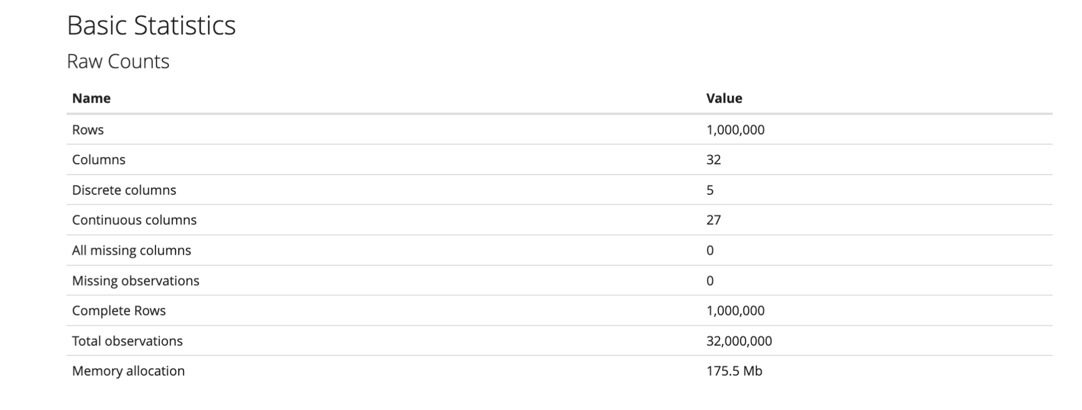
Each dataset consists of 1 million instances with 32 realistic features used in fraud detection, including a column for “month” (temporal information) and protected attributes such as age group, employment status, and income percentage.

Features

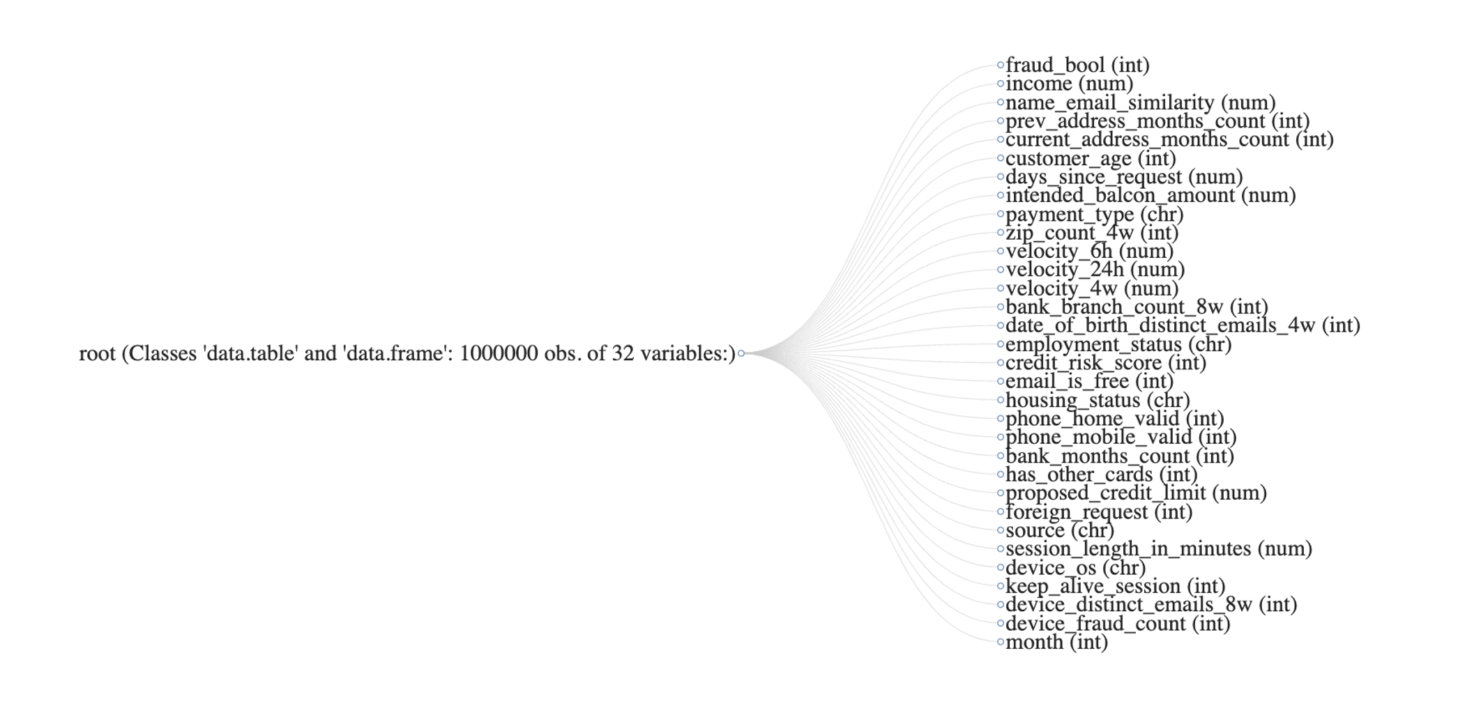
The dataset includes features that are critical to understanding the patterns behind fraudulent transactions. These features include but are not limited to:

Feature Description

Feature	Description
Fraud label	Indicator of fraudulent transaction
Annual income of the applicant	Income of the applicant for a specific year
Similarity between email and applicant’s name	How closely the applicant’s name matches their email address
Number of months in previous registered address	Duration of stay at the previous address
Months in the currently registered address	Duration of stay at the current address
Applicant’s age	Age of the applicant
Number of days passed since the application was made	Time elapsed since the application was submitted
Initial transferred amount for application	Initial amount transferred when application was made
Credit payment plan type	Type of the credit payment plan
Number of applications within the same zip code in the last 4 weeks	Applications count in the same zip code in the last 4 weeks
Velocity of total applications made in various time frames	Speed at which applications are being made
Number of total applications in the selected bank branch in the last 8 weeks	Total applications in a specific branch in the last 8 weeks
Number of emails for applicants with the same date of birth in the last 4 weeks	Number of emails for same birthdate applicants in the last 4 weeks
Employment status of the applicant	Applicant’s current employment status
Internal score of application risk	Risk score given to the application by the bank
Domain of application email	Domain type of the applicant’s email (free or paid)
Current residential status for the applicant	Current housing situation of the applicant
Validity of provided phones	Whether the provided phone numbers are valid
How old is the previous account (if held) in months	Age of the previous account (if any)
If the applicant has other cards from the same banking company	Whether the applicant has other cards from the same bank
Applicant’s proposed credit limit	Credit limit proposed by the applicant
If the origin country of the request is different from the bank’s country	Whether the application is from a different country
Online source of application (browser or mobile app)	Where the application was made (browser or mobile app)
Length of user session on the banking website	Duration of the user’s session on the bank’s website
Operating system of the device that made the request	OS of the device used to make the request
User option on session logout	User’s action when logging out
Number of distinct emails from the used device in the last 8 weeks	Unique email counts from the device in the last 8 weeks
Number of fraudulent applications with the used device	Count of fraudulent applications made from the device
Month where the application was made	Month of application submission

Hive queries analysis

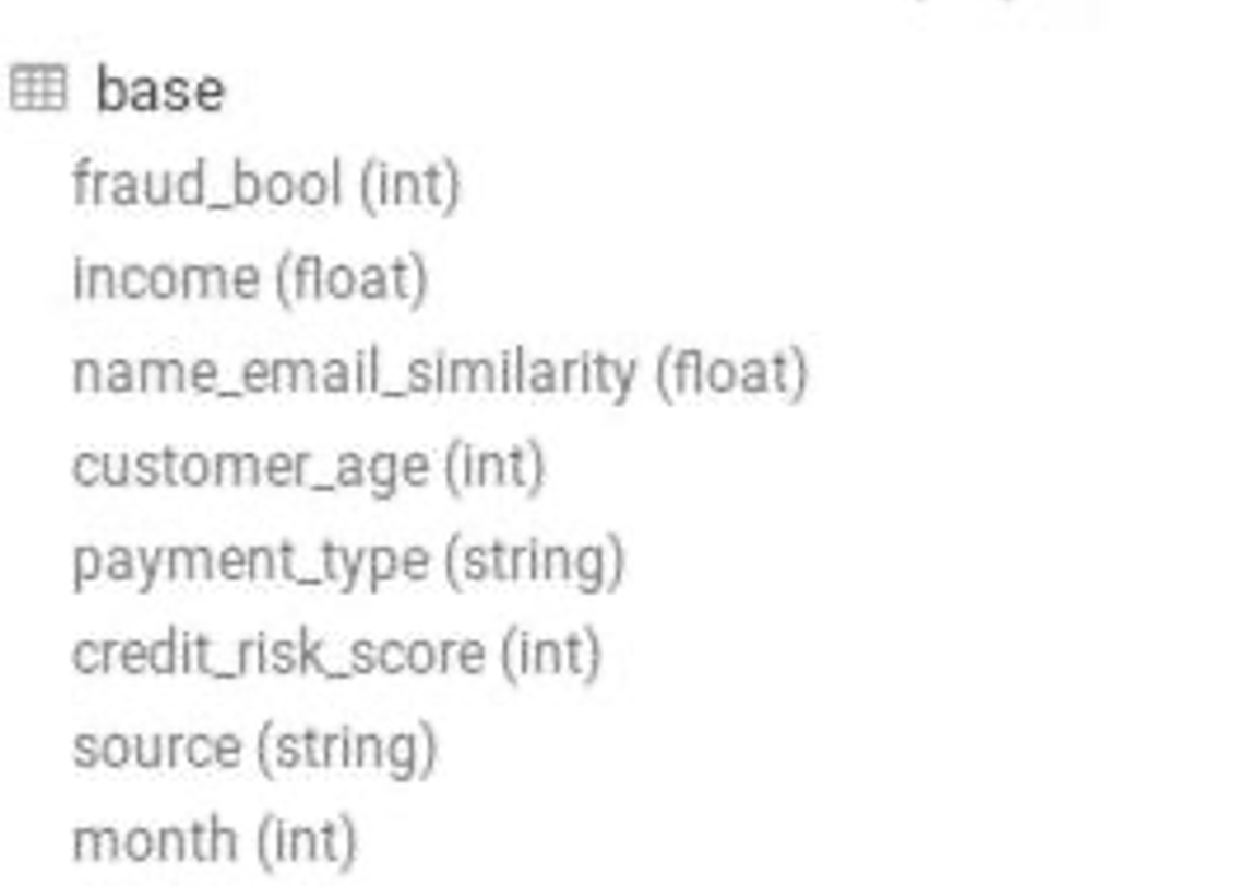
The Base_table CSV file was imported into HDFS from the local machine using Hive File browser. An external Hive table was created using the file location. The table contains several columns including fraud_bool, income, name_email_similarity, customer_age, payment_type, credit_risk_score, source, and month. There are a total of 201,612 records in the table.

CREATE EXTERNAL TABLE Base (
fraud_bool INT,
income FLOAT,
name_email_similarity FLOAT,
customer_age INT,
payment_type STRING,
credit_risk_score INT,
source STRING,
month INT
)
ROW FORMAT DELIMITED
FIELDS TERMINATED BY ','
STORED AS TEXTFILE
LOCATION ‘/User/cloudera/';

Question: How many customers of each age have a fraud bool of 1?

SELECT customer_age, COUNT(\*)
FROM Base
WHERE fraud_bool = 1
GROUP BY customer_age;

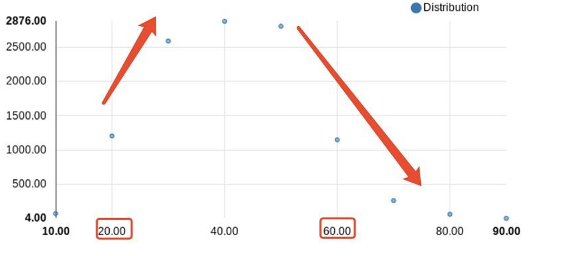
The analysis shows a clear trend in the relationship between age and likelihood of fraudulent activities. Customers in the age bracket of 10 to 40 years show an increasing likelihood of fraud, with the peak incidence at age 40. Beyond the age of 40, the likelihood of fraudulent activities begins to decline. This trend could suggest that individuals in their prime working years have a higher tendency to be associated with fraudulent activities. We should consider this age-related trend in the development of our risk models and fraud detection systems, while remaining mindful of the multifaceted nature of fraudulent behavior.

This trend could suggest that individuals in their prime working years have a higher tendency to be associated with fraudulent activities.

Question: How does income relate to the likelihood of fraud?

SELECT income, AVG(fraud_bool) as avg_fraud
FROM Base
GROUP BY income
ORDER BY income;

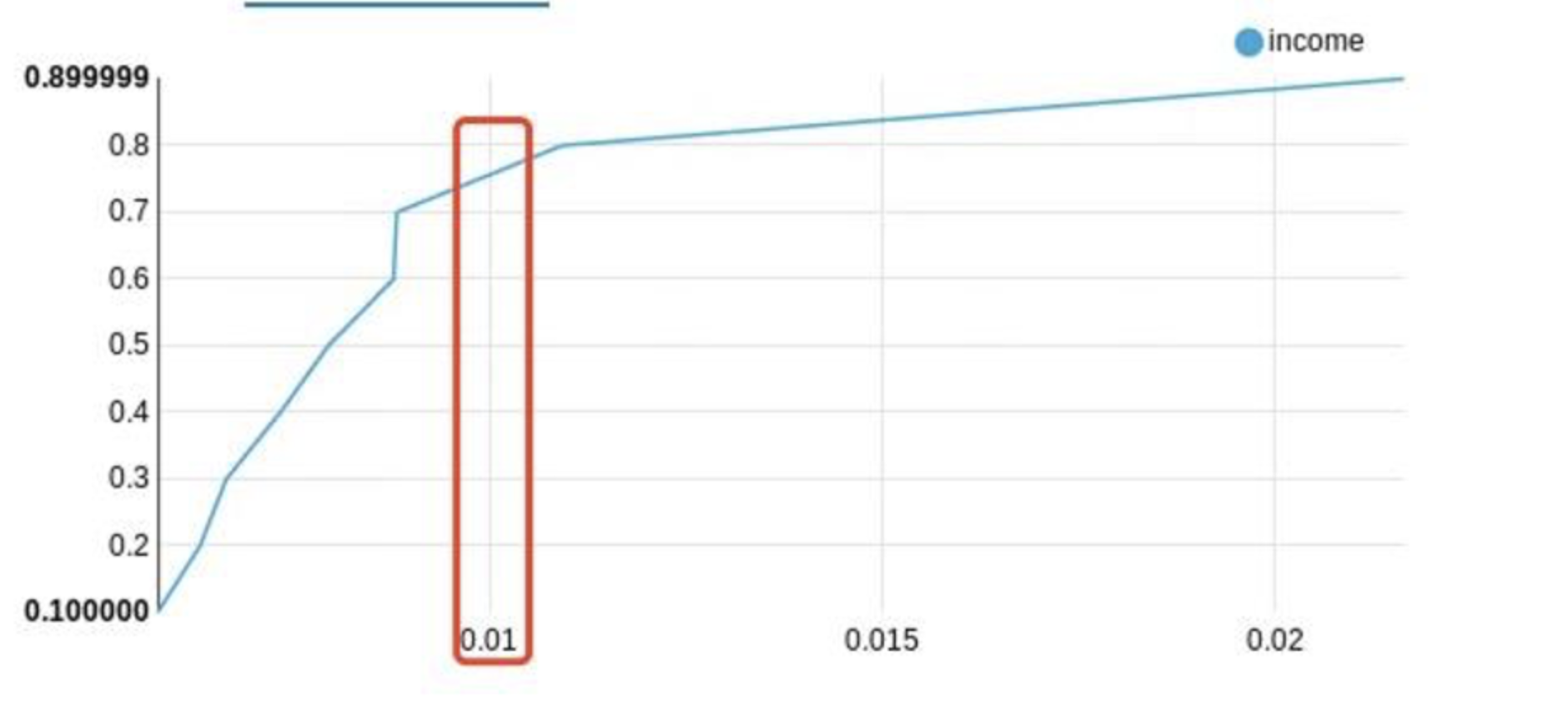
This question and query can provide insights on whether higher or lower incomes are associated with higher rates of fraudulent activity. The output can be plotted on a graph, where the x-axis represents average fraud rate and the y-axis represents the income. This suggests that higher-income individuals are more likely to be associated with fraudulent activities. It’s important to interpret this cautiously; while income can be a significant factor, it’s among several other indicators that contribute to fraud risk. We recommend incorporating this finding into our risk models to enhance fraud detection and prevention measures, while simultaneously considering other crucial variables.

We can see from this plot that higher-income individuals are more likely to be associated with fraudulent activities.

Question: What’s the distribution of payment types among fraudulent transactions?

SELECT payment_type, COUNT(\*) as num_frauds
FROM Base
WHERE fraud_bool = 1
GROUP BY payment_type
ORDER BY num_frauds DESC;

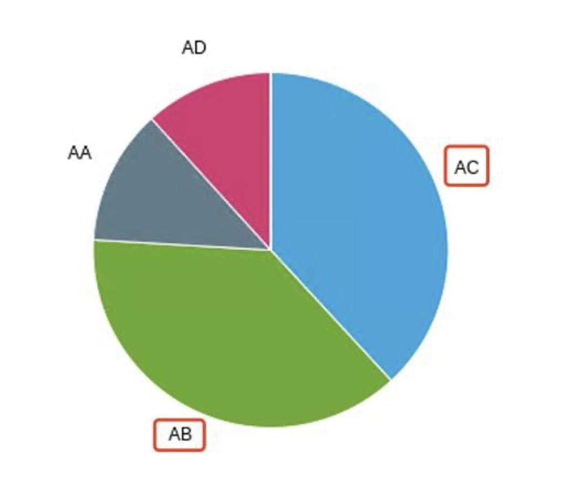
The pie chart shows a diversity in fraudulent activities across different payment types. Notably, “AB” tops the chart with the largest fraction of frauds. It is closely followed by “”AC”.

Question: What are the different sources of transactions and how do they relate to the fraud rate?

SELECT source, AVG(fraud_bool) as avg_fraud
FROM Base
GROUP BY source
ORDER BY avg_fraud DESC;

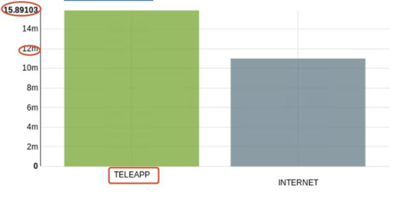
Analysis shows that transactions made through teleapp have a higher fraud rate than those conducted via the internet. This suggests teleapp transactions could be more vulnerable to fraud, warranting additional scrutiny or security measures to mitigate potential fraudulent activities.

Question: What’s the monthly trend of fraudulent transactions?

SELECT month, COUNT(\*) as num_frauds
FROM Base
WHERE fraud_bool = 1
GROUP BY month
ORDER BY month;

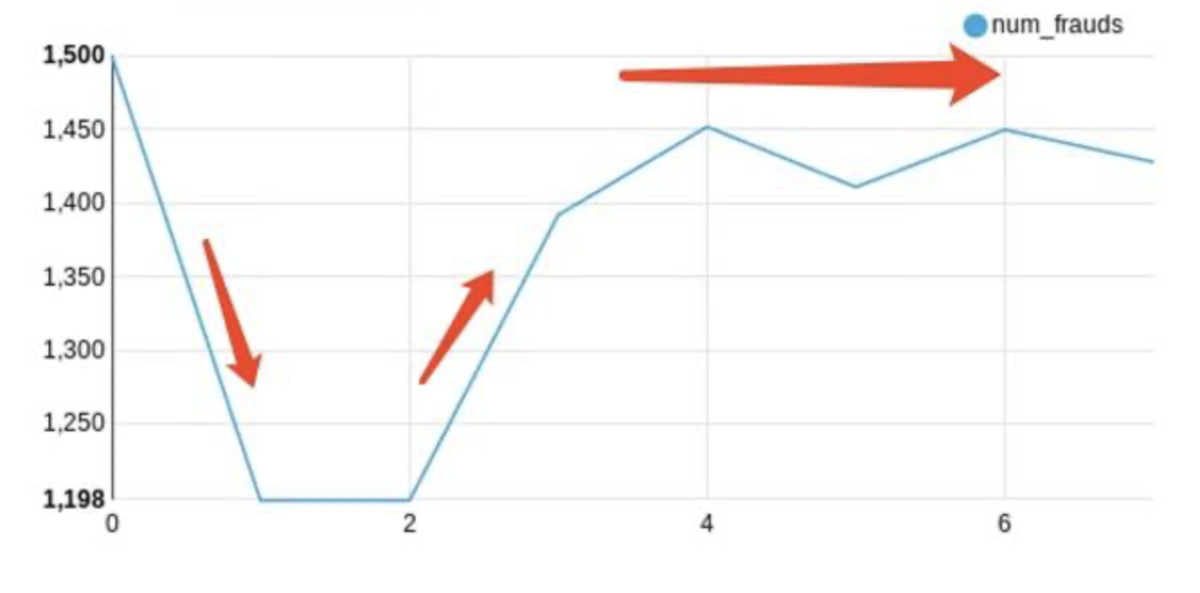
Our analysis shows a clear monthly trend in fraudulent transactions. The beginning of the year sees a lower rate of fraud, which significantly increases from March onwards. This suggests that heightened vigilance and preventive measures may be necessary during this latter period to mitigate potential fraud.

Clustering

The primary objective of this study is to identify significant clustering, correlations, and patterns in our extensive customer database. This process will allow us to better understand the factors that contribute to fraudulent activities and consequently develop preventive strategies.

Our analysis is based on a dataset consisting of one million customers. Each customer record includes various attributes such as income, credit risk score, housing status, number of months at the current address, number of months at the previous address, age, days since the last request, and more. In total, we have more than 20 distinct attributes, each providing a different perspective on customer behavior.

The crucial part of the data is the ‘fraud_bool’ field, which indicates whether a transaction made by the customer was fraudulent (1) or not (0). Our primary aim is to detect patterns that increase the likelihood of fraud based on other attributes.
To uncover these patterns, we use methods of descriptive statistics, correlation analysis, and clustering techniques. Descriptive statistics provide an initial insight into data, correlation analysis points out the relationships between variables, and clustering helps group similar customers, making the patterns easier to understand and interpret.

Ultimately, our goal is to develop a comprehensive understanding of the factors that increase the risk of fraudulent transactions. This understanding will serve as a basis for developing preventive strategies and, if applied effectively, could significantly reduce the prevalence of fraud in our customer transactions. This contribution will enhance our risk management strategies and ensure a safer environment for our customers.

In conclusion, our methodology involves comprehensive data analysis to identify critical patterns and correlations in our customer data, aiming to improve our fraud detection and prevention capabilities significantly.

How and when:

Data Acquisition and Preprocessing with Hadoop: We procure a dataset of one million customer records from our database. This dataset, which forms the foundation for our analysis, is aimed at identifying significant correlations, patterns, and clusters in the data related to fraudulent transactions. We use Hadoop’s distributed file system (HDFS) to store and process our large dataset. This involves cleaning the data and dealing with missing or anomalous values, tasks which can be efficiently accomplished using Hadoop’s MapReduce paradigm.

Exploratory Data Analysis: An initial descriptive statistical analysis is performed to understand the basic characteristics of the data. It involves calculating measures such as mean, median, minimum, maximum, and standard deviation for each variable in the dataset.

Correlation Analysis: We perform correlation analysis to uncover any significant relationships between the different customer attributes. This step is crucial for understanding which variables might be influencing the ‘fraud_bool’ outcome.

Clustering Model Development and Evaluation with Spark: The preprocessed data is then loaded into Apache Spark for analysis. We first perform exploratory data analysis using Spark to understand the basic characteristics of our data. Following this, we use Spark’s Machine Learning Library (MLlib) to conduct a correlation analysis, revealing significant relationships between different customer attributes. To identify customer clusters with high rates of fraudulent transactions, we apply a clustering algorithm, also available in Spark’s MLlib. The performance of our model is then evaluated and iterated upon until we achieve satisfactory results.

Strategies Development and Deployment: Based on our insights, we develop strategies to prevent fraudulent transactions. This could include stricter checks for specific clusters of customers or tailoring our fraud detection models to consider the patterns identified in this study. Our strategies are then deployed and continuously monitored for effectiveness.

Throughout the process, we will iterate and refine our methods as needed, continuously learning from our data to improve our ability to detect and prevent fraudulent transactions.
Real-world Example
Problem:

The surge in digital transactions has brought along an unwanted companion - fraud. It poses a daunting challenge to both financial institutions and regulatory bodies. The pertinent question we aim to address is: “How can we leverage machine learning to predict and mitigate fraudulent transactions in banking?”

Goal：

The goal here is to develop a clustering model to detect and flag potentially fraudulent transactions. These models will examine specific elements of customer transactions and behavior such as transaction amount, time, location, and customer’s past behavior patterns, etc. The aim of this task is to accurately categorize transactions into ‘normal’ and ‘suspicious’ clusters, enhancing our business’s safety and protecting our customers from potential financial loss.

Business Question:

● What percentage of transactions are fraudulent?

● Fraudulent with age relationship?

● Fraudulent with annual income relationship?

● Are there specific transaction types that are more likely to be fraudulent? Can we identify any patterns or trends in fraudulent transactions over time?

● Does the source of the transaction (TELEAPP vs INTERNET) have an impact on the likelihood of it being fraudulent?

● What is the relationship between the similarity of names and emails and the frequency of fraudulent transactions?

● How does the housing status affect the likelihood of fraudulent transactions?

● How does employment status affect the average credit risk score and the occurrence of fraudulent transactions?

● Are there any geographic patterns in fraudulent transactions? Are certain regions more prone to fraud than others? Fraudulent Transactions & Zipcode

● Are there specific times of the day, days of the week, or months of the year when fraudulent transactions are more common?

Methodology：The general approach would involve the following steps:

Data Collection:

Assemble a dataset of customer transactions from our business. The more varied the dataset, the better the model will perform on unseen data.
● Load the Data

To begin, we must first load the data into our working environment. In R, we can accomplish this by utilizing the read.csv() function. The code is as follows:
df <- read.csv("path_to_your_file/Base.csv")
This code reads the CSV file, “Base.csv,” from the specified path and loads it into the data frame ‘df’ for further manipulation and analysis.

Pre-processing:

This involves cleaning up the data, which may involve handling missing data, outlier detection, feature scaling, and other data normalization processes.

Data Cleaning:

After loading the data, the next crucial step is data cleaning. This process involves handling missing values, detecting outliers, and ensuring that the data is in the correct format for analysis. It’s a critical step as the quality of data and the validity of statistical inference from that data depend heavily on the extent to which it is ‘clean’.

Feature Engineering:

Define a set of features that are relevant to the problem at hand, such as 'Transaction Amount', 'Transaction Time', 'Customer Past Behavior', 'Location', etc. These features form the input to our clustering model.

Business Questions And Exploratory Data Analysis (EDA):

With a clean dataset, we can then perform our analysis to discover clusters, correlations, and patterns.

● What percentage of transactions are fraudulent?

1 if fraud, 0 if legit

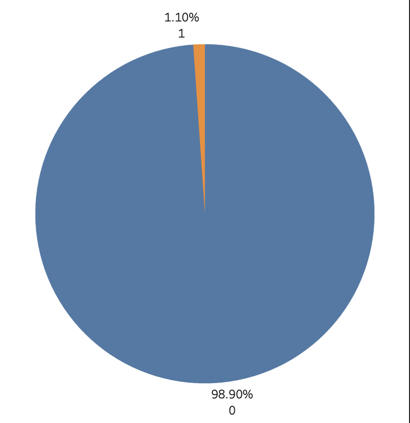
In analyzing the distribution of transactions in the dataset, it is observed that a small fraction of the transactions are fraudulent. Specifically, from the pie chart, it is evident that fraudulent transactions constitute approximately 1.1% of the total transactions. The overwhelming majority, which is 98.9%, are non-fraudulent transactions. This indicates that while fraud is present, it represents a relatively minor portion of the overall transaction activity. It is crucial for businesses and financial institutions to remain vigilant and employ robust fraud detection mechanisms to identify and mitigate these fraudulent transactions, despite their scarcity, to ensure the security and integrity of financial operations.

● Fraudulent with age relationship?

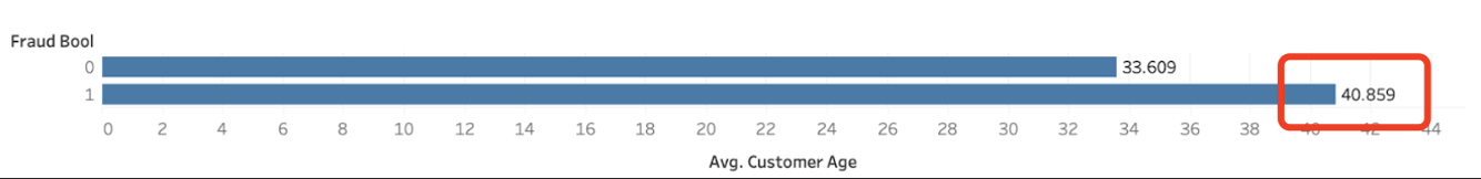
The dataset reveals a notable relationship between age and the likelihood of a transaction being fraudulent. On average, fraudulent transactions are associated with an older age group, with the average age being 40 years old. In contrast, non-fraudulent transactions are associated with a younger demographic, having an average age of 33 years old.

● Fraudulent with annual income relationship?

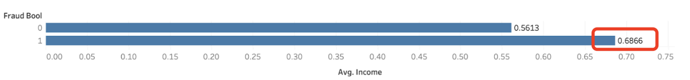
The annual income of the applicant in quantiles. Ranges between [0, 1].

The plot indicates a relationship between the annual income of the applicant and the likelihood of a transaction being fraudulent.

The annual income is represented in quantiles, ranging from 0 to 1, where a higher value represents a higher income.

On average, non fraudulent transactions are associated with a lower annual income quantile, with an average value of 0.56.

Conversely, fraudulent transactions are associated with a higher annual income quantile, having an average value of 0.67.

This suggests that individuals with relatively higher annual incomes are more likely to be involved in fraudulent transactions compared to those with lower incomes.

●Are there specific transaction types that are more likely to be fraudulent? Can we identify any patterns or trends in fraudulent transactions over time?

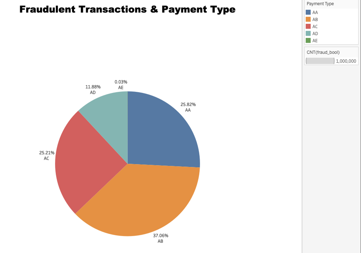
Based on the data provided in the pie chart, we can infer that different payment types have varying levels of fraudulent activities. The payment type “AB” stands out with the highest percentage of fraudulent transactions, accounting for 37.0554% of the total fraudulent activities. This is followed by payment type “AA” with 25.8249%, payment type “AC” with 25.2071%, and “AD” with 11.8837%. The payment type “AE” had the least fraudulent activities, accounting for only 0.0289% of the total count.

● Does the source of the transaction (TELEAPP vs INTERNET) have an impact on the likelihood of it being fraudulent?

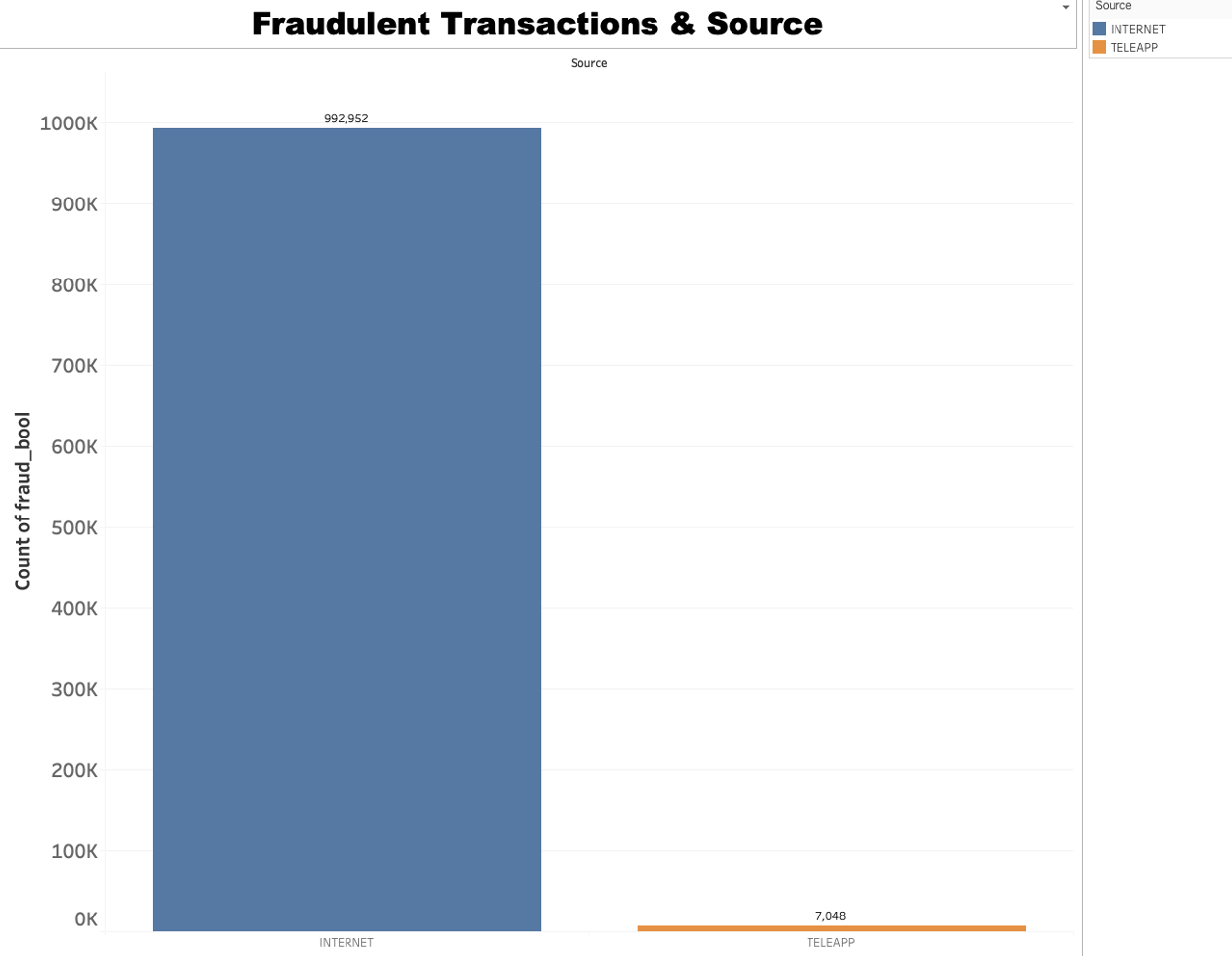
From the plot, it’s clear that the count of fraudulent transactions varies significantly based on the transaction source. There are far more fraudulent transactions originating from the INTERNET (992,952) than from TELEAPP (7,048).

● What is the relationship between the similarity of names and emails and the frequency of fraudulent transactions?

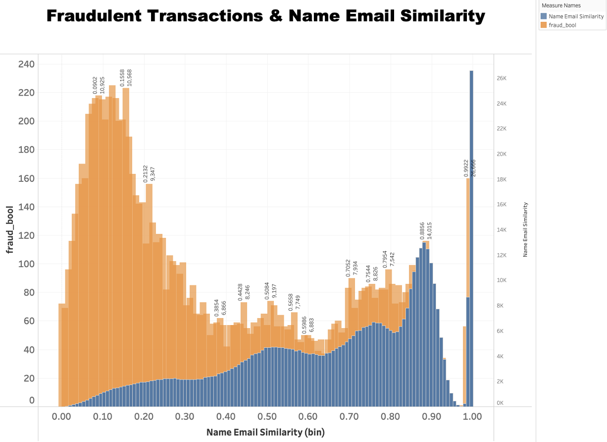
The dual histogram indicates an interesting correlation between the similarity of name and email and fraudulent transactions. As the name-email similarity score ranges from 0 to 1, where a higher score indicates a higher similarity, the number of fraudulent transactions displays a clear trend.

Initially, the count of fraudulent transactions is relatively low when the name-email similarity is less than 0.1. As the similarity score increases, specifically from 0.1 to about 0.9, the count of fraudulent transactions also shows a significant increase. This implies that transactions are more likely to be fraudulent when there is a moderate to high similarity between the name and email.
However, the pattern is not monotonically increasing. When the similarity score goes beyond 0.9, the number of fraudulent transactions drops sharply. Specifically, it falls dramatically after the similarity score surpasses 0.95 and stays low until the score reaches around 0.984. After that, the count of fraudulent transactions surges, reaching its peak at a similarity score of approximately 0.992.

● How does the housing status affect the likelihood of fraudulent transactions?

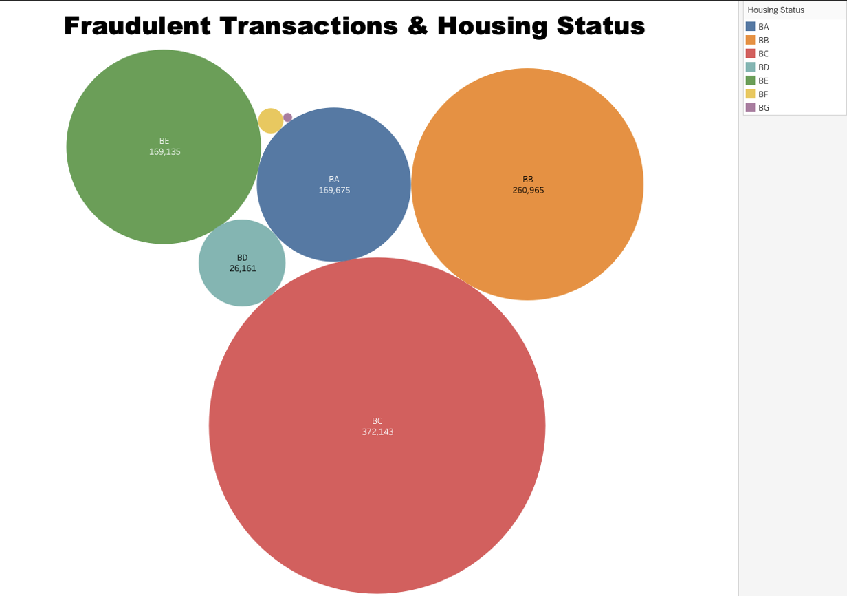
The stacked bar chart represents the relationship between housing status and fraudulent transactions. Different housing statuses are categorized from ‘BA’ to ‘BG’, and each category displays the count of fraudulent transactions, the number of days since request, and the ‘fraud_bool’ which probably indicates a boolean variable for whether a transaction is fraudulent or not.

➢ ‘BG’ status had 252 fraudulent transactions over 352.8 days, with a fraud_bool value of 1.

➢ ‘BF’ status reported 1,669 fraudulent transactions over 2,763.9 days, with a fraud_bool of 7.

➢ ‘BD’ status witnessed 26,161 fraudulent transactions over 32,739.5 days, with a fraud_bool of 226.

➢ ‘BE’ status recorded 169,135 fraudulent transactions over 163,782.6 days, and a fraud_bool of 582.

➢ ‘BA’ status had a massive rise to 169,675 fraudulent transactions over 102,903.6 days, with a fraud_bool of 6,357.

➢ Finally, ‘BB’ and ‘BC’ statuses reported 260,965 and 372,143 fraudulent transactions respectively, over certain durations, with fraud_bool values of 1,568 and 2,288.

In conclusion, housing status influences the count of fraudulent transactions, but a higher count does not necessarily mean a higher percentage of fraudulent transactions, as indicated by the fraud_bool values.

● How does employment status affect the average credit risk score and the occurrence of fraudulent transactions?

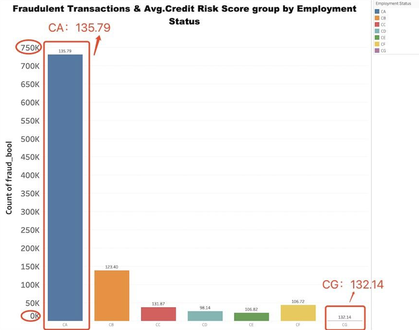
The bar plot shows the relationship between employment status, the average credit risk score, and the number of fraudulent transactions.

➢ ‘CA’: The highest score at 135.79, and a massive fraud count at 730,252.

➢ ‘CG’: A similar score of 132.14, but significantly fewer fraud cases at 453.

➢ ‘CD’: An average credit risk score of 98.14 and 26,522 fraudulent transactions.

➢ ‘CF’: Credit score of 106.72, and fraud count is 44,034.

➢ ‘CE’: Score is 106.82, with 22,693 fraud cases.

➢ ‘CB’: The score jumps to 123.40, and fraud count to 138,288.

➢ ‘CC’: Score increases to 131.87, yet fraud drops to 37,758.

The plot indicates a complex relationship between employment status, credit risk score, and fraudulent transactions. Higher credit scores do not necessarily equate to more fraud cases, as shown by the ‘CG’ and ‘CA’ statuses.

● What is the relationship between the average number of fraudulent transactions, the average customer age, and the type of device operating system they use?

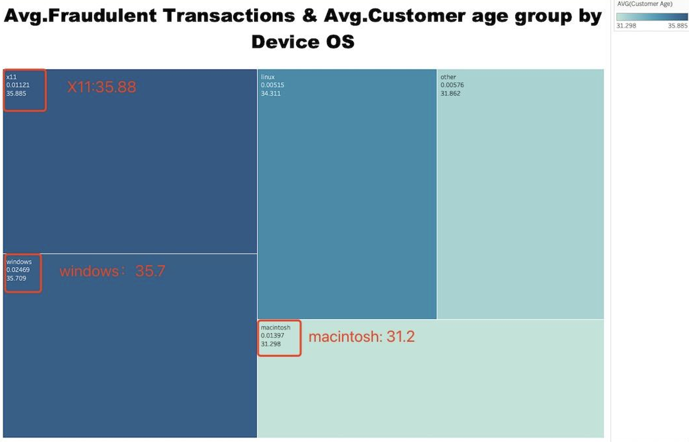
The heatmap analysis shows how the average age of customers and average number of fraudulent transactions differ based on the device operating system:

➢ X11: Users have the highest average age of 36 years, and a moderate fraud rate at 0.01121.

➢ Windows: The average customer age is even higher at 36 years, and it also has the highest fraud rate at 0.02469.

➢ Macintosh: The average customer age is around 31 years and the average rate of fraudulent transactions is 0.01397.

➢ Other OS: Average customer age is slightly higher at 32 years, while the average fraud rate is lower at 0.00576.

➢ Linux: Users are older with an average age of 34 years and have a relatively low fraud rate at 0.00515.

From this, we see that different device OS are associated with different customer ages and fraud rates. Windows, despite having an older average user base, experiences the highest rate of fraudulent transactions.

● Are there any geographic patterns in fraudulent transactions? Are certain regions more prone to fraud than others? Fraudulent Transactions & Zipcode

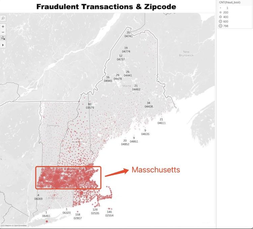
From above plots. In Massachusetts, we observe the highest and most concentrated instances of fraudulent transactions. A multitude of postal code areas display significant counts of fraudulent activity. For example, the 01749 postal code area reports 281 fraudulent transactions, 01740 has 327, 01522 records 391, and 01473 notes an alarming 452 fraudulent transactions.
In Rhode Island, the number of fraudulent transactions is slightly less than in Massachusetts but still considerably high. For example, the 02904 postal code area has 103 fraudulent transactions, the 02912 area has 108, the 02907 area has 140, and the 02863 area has 142.

In New Hampshire, the number of fraudulent transactions reduces further but remains significant. For instance, the 03816 postal code area has 42 fraudulent transactions, the 03245 area has 81, the 03247 area has 86, and the 03299 area has 98.

In Vermont, the number of fraudulent transactions reduces further, with most areas seeing less than 10 fraudulent transactions. For instance, the 05401 and 05451 postal code areas each have 6 fraudulent transactions, the 05446 area has 8, the 05406 area has 10, and the 05407 area has 15.

In Maine, the number of fraudulent transactions is also low but slightly higher than in Vermont. For example, the 04984 postal code area has 12 fraudulent transactions, the 04221 area has 24, the 04228 area has 31, and the 04266 area has 49.

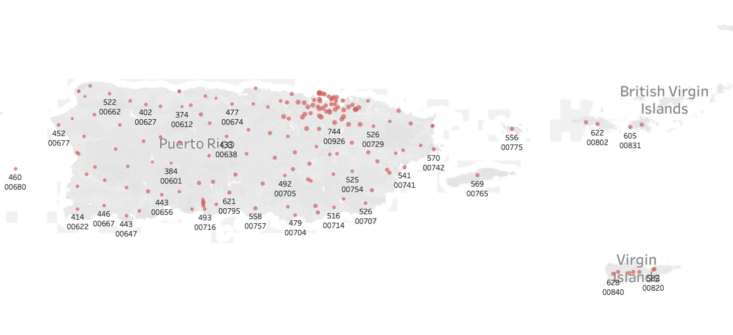
In Puerto Rico, fraudulent transactions are highly prevalent but not densely concentrated. Postal codes 00646, 00902, 00979, and 00910 report 439, 650, 671, and 684 fraudulent transactions respectively, suggesting a widespread rather than localized issue.

Though the number of fraudulent transactions in other areas like Rhode Island, New Hampshire, Vermont, Maine, and Puerto Rico is also noteworthy, none match the density and intensity of fraudulent activity seen in Massachusetts. This implies that while fraudulent transactions are a universal issue, they are particularly prevalent in Massachusetts, thus necessitating further investigation and preventative measures in the state.

● Are there specific times of the day, days of the week, or months of the year when fraudulent transactions are more common?

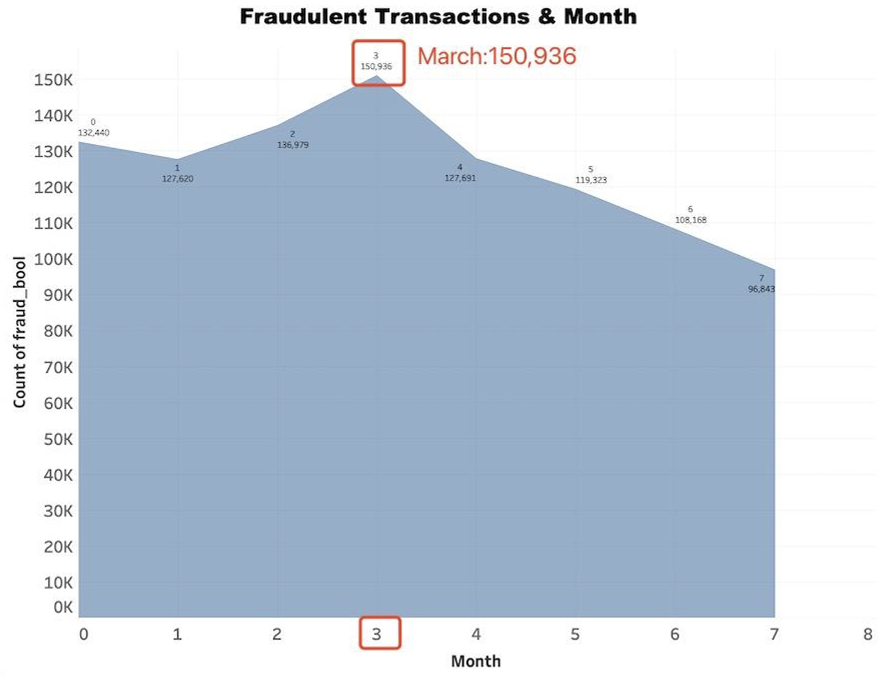
The area plot demonstrates the correlation between the month and the number of fraudulent transactions:

➢ In the month of July (7), there were 96,843 fraudulent transactions.

➢ In June (6), there were 108,168 fraudulent transactions.

➢ May (5) saw a further increase to 119,323 fraudulent transactions.

➢ In January (1), the count reached 127,620 fraudulent transactions.

➢ April (4) had a similar count, with 127,691 fraudulent transactions.

➢ February (2) experienced a rise in fraudulent transactions, with a total of 136,979.

➢ Finally, March (3) had the highest count of fraudulent transactions, with a total of 150,936.

From this plot, we can see that the number of fraudulent transactions tends to increase over the months, with March reporting the highest number. This may suggest that the time of the year influences the occurrence of fraudulent transactions.

Correlations Analysis：

Is there a correlation between the transaction amount and the likelihood of fraud? Are there any other correlations in the data that could help predict fraud?

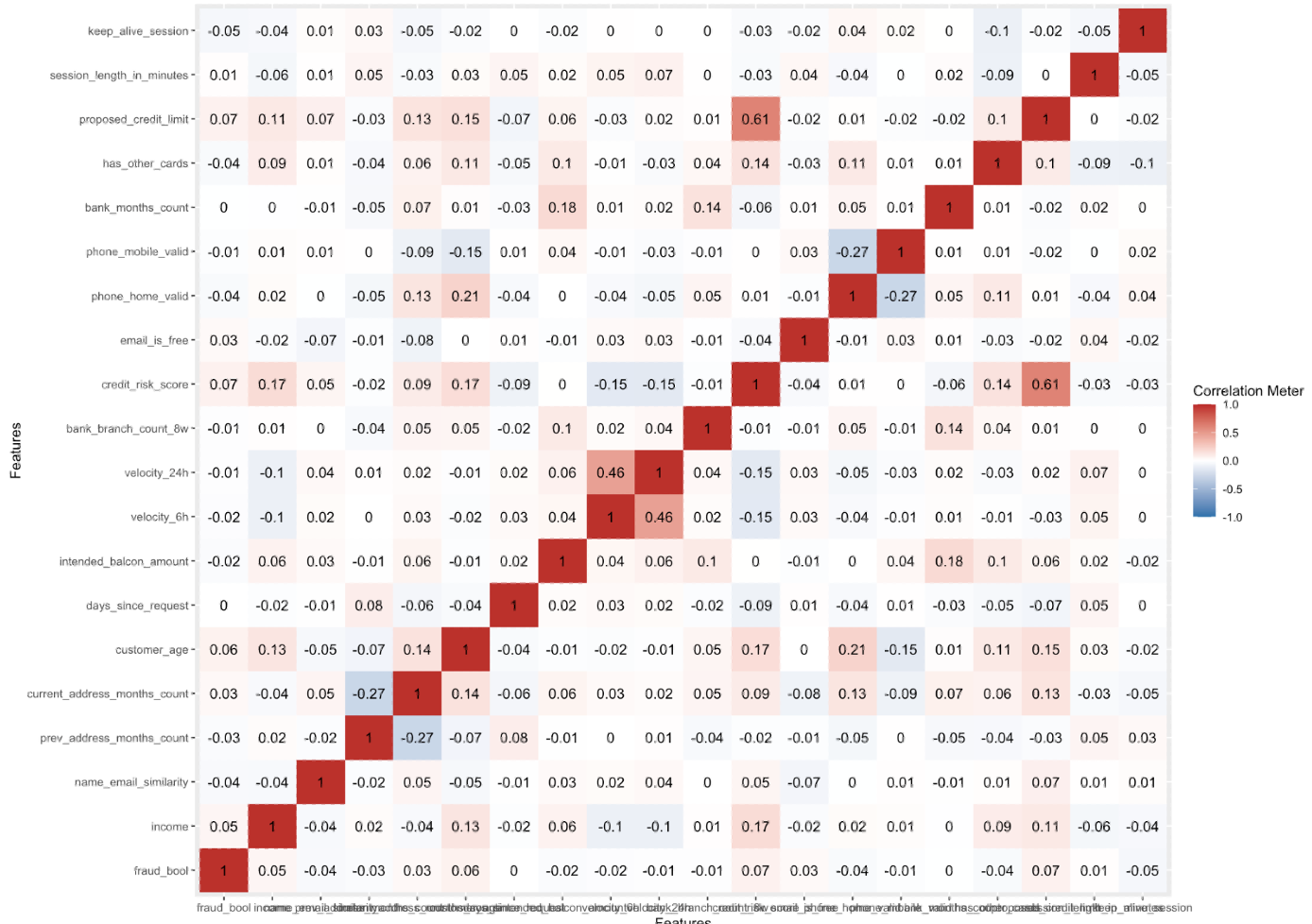
This report analyzes the correlation between various features in a dataset related to bank account fraud. The dataset includes features such as fraud_bool, income, name_email_similarity, prev_address_months_count, and others. Correlation coefficients range from -1 to 1, where -1 indicates a perfect negative correlation, 1 indicates a perfect positive correlation, and 0 indicates no correlation.

I. Fraud and Credit Risk Score: There is a positive correlation between fraud_bool and credit_risk_score (0.071), suggesting that as the credit risk score increases, the likelihood of fraud also increases, though the correlation is weak.

II. Fraud and Customer Age: There is a weak positive correlation between fraud_bool and customer_age (0.063), indicating that older customers are slightly more likely to be involved in fraud.
III. Income and Credit Risk Score: There is a positive correlation between income and credit_risk_score (0.171), suggesting that individuals with higher income tend to have higher credit risk scores.

IV. Income and Customer Age: There is a positive correlation between income and customer_age (0.126), indicating that older individuals tend to have higher incomes.

V. Name-Email Similarity and Current Address Months Count: There is a positive correlation between name_email_similarity and current_address_months_count (0.050), suggesting that individuals with more similar names and emails tend to have lived at their current address for longer.

VI. Previous and Current Address Months Count: There is a strong negative correlation between prev_address_months_count and current_address_months_count (-0.272), indicating that individuals who have lived at their previous address for a longer time tend to have lived at their current address for a shorter time.

VII. Credit Risk Score and Proposed Credit Limit: There is a strong positive correlation between credit_risk_score and proposed_credit_limit (0.606), suggesting that individuals with higher credit risk scores are likely to have higher proposed credit limits.

VIII. Keep Alive Session and Fraud: There is a weak negative correlation between keep_alive_session and fraud_bool (-0.050), suggesting that fraud is less likely to occur in sessions that are kept alive.

Model Training&Clustering Analysis:

Use a clustering algorithm (like K-means, DBSCAN, or Hierarchical clustering) to learn from this data. The algorithm forms clusters of transactions based on similarities and dissimilarities among the input features.
● **Load libraries:**The sparklyr library is used for connecting to Apache Spark, dplyr is used for data manipulation, cluster is used for cluster analysis, and ggplot2 is used for visualization.

# Load libraries
library(sparklyr)
library(dplyr)
library(cluster)
library(ggplot2)

● Connect to Spark: A connection is established to Apache Spark using the spark_connect() function.

# Connect to Spark

Sys.setenv(SPARK_HOME="/Users/mac/Desktop/spark-3.4.0-bin-hadoop3")
sc <- spark_connect(master = "local")
● Load data: The Base data is loaded into a Spark DataFrame using read.csv() function and then transferred to Spark using copy_to() function.

# Load data

setwd('/Users/mac/Desktop/A-school/3-6110')
Base <- read.csv('Base.csv')
Base_tbl <- copy_to(sc, Base, "Base", overwrite = TRUE) # overwrite the same table if it exists

● Select the relevant variables: We use dplyr’s select() function to choose the relevant variables from the Base data frame and store them in a new data frame df_selected.

# Continue to use Base_tbl as the Spark dataframe (tbl)

df_selected <- Base_tbl %>%
select(income, credit_risk_score, days_since_request, proposed_credit_limit, customer_age)
● Normalize the data: This step is crucial for clustering as it ensures all variables contribute equally to the analysis. Variables with larger scales could dominate the clustering otherwise. The scale() function standardizes the variables to have a mean of 0 and standard deviation of 1.

# Normalize my data

df_selected <- sdf_scale(df_selected)

● Handle missing values: Here, any rows with missing data are removed using na.omit(). An alternative approach might be to fill missing values with some value (like mean or median), but that’s not done here.

# Check for missing values and handle them appropriately

df_selected <- df_selected %>%
filter(!is.na(income), !is.na(credit_risk_score), !is.na(days_since_request), !is.na(proposed_credit_limit), !is.na(customer_age))
● K-means clustering: Using the kmeans() function, we perform k-means clustering on df_selected. The set.seed(123) is used for reproducibility.

# K-means clustering

set.seed(123) # for reproducibility
k <- 6
km_result <- ml_kmeans(df_selected, centers = k, features = colnames(df_selected))

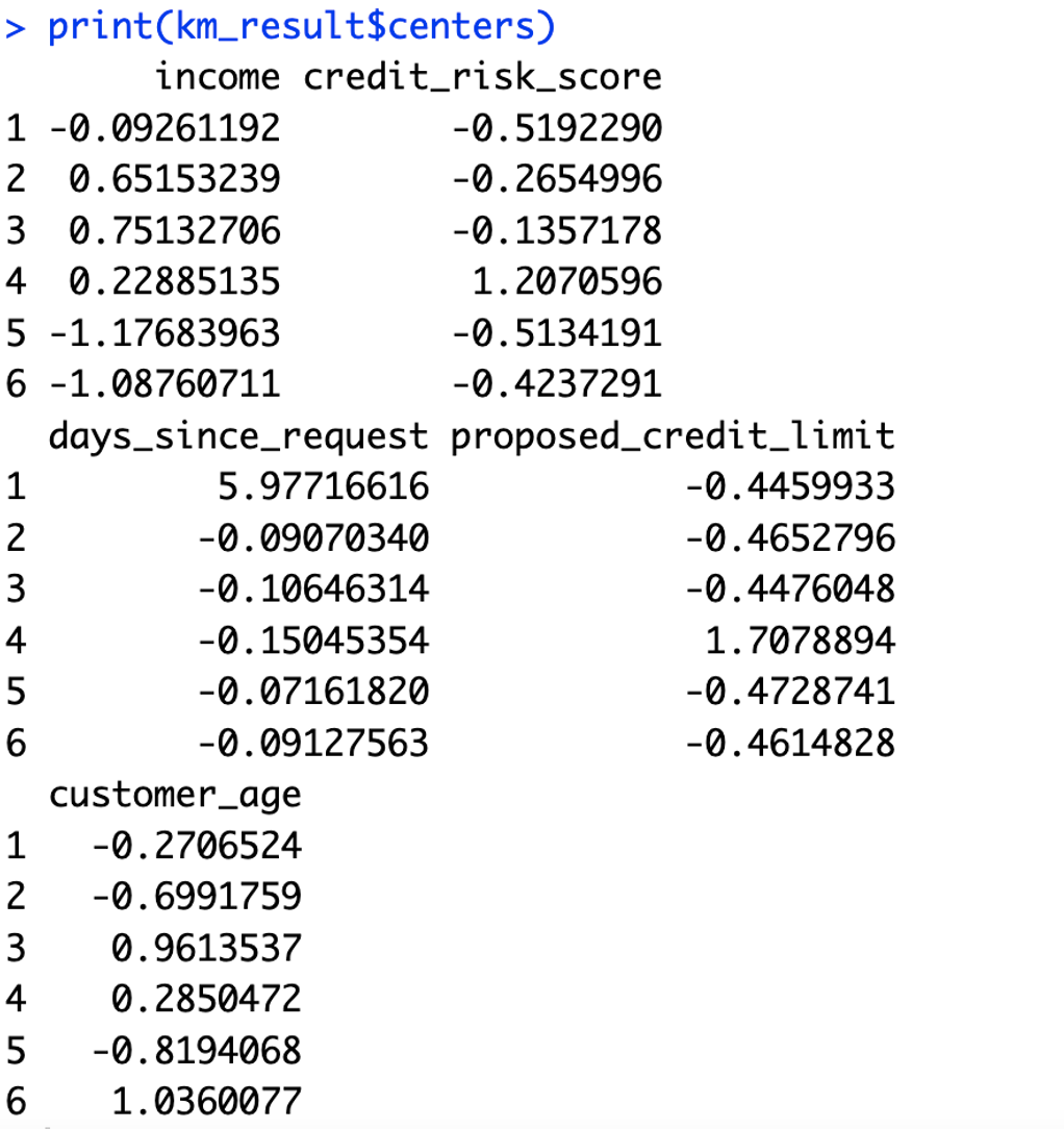
● Check the cluster sizes and centers: The script prints the sizes of the clusters (i.e., how many observations each cluster contains) and the cluster centers (i.e., the mean value of each variable in each cluster).

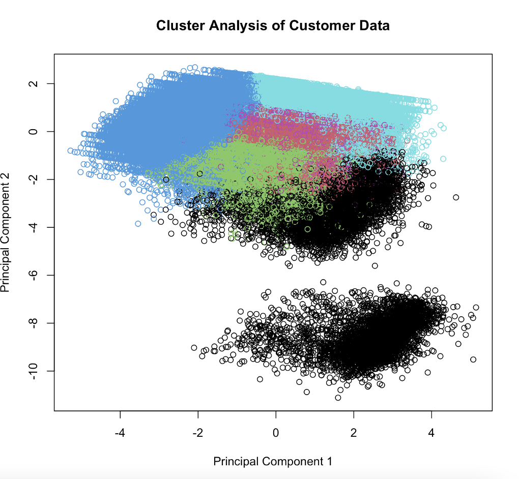
● Apply PCA to reduce dimensions: Principal Component Analysis (PCA) is used to reduce the dimensionality of the data, making it easier to visualize. PCA finds a new set of dimensions such that all the dimensions are orthogonal (uncorrelated) and capture the maximum amount of variation in the data.

# ApplyPCA for visualization

df_tbl <- sdf_predict(km_result, df_selected) %>% collect()
pca <- prcomp(unlist(df_tbl$features), center = TRUE, scale. = TRUE)
pca_df <- data.frame(principal_component_1 = pca$x[, 1], principal_component_2 = pca$x[, 2], cluster = df_tbl$prediction)

● Plotting the clusters: The km_result$centers output shows the center (mean value) of each cluster for each variable. To make it clearer, let’s plot it. A scatter plot of the first two principal components is created. Each point represents an observation in the data and is colored according to the cluster it belongs to.

ggplot(pca_df, aes(x = principal_component_1, y = principal_component_2)) +
geom_point(aes(color = as.factor(cluster))) +
labs(color = "Cluster", title = "Cluster Analysis of Customer Data", x = "Principal Component 1", y = "Principal Component 2")

Cluster 1: These are customers with slightly below-average income and much lower than average credit risk score. They requested their credit a very long time ago (significantly higher than average days since request) and have a much lower than average proposed credit limit. They are slightly younger than the average customer.

Cluster 2: These are customers with significantly above-average income and below-average credit risk score. They recently requested their credit (below-average days since request) and have a lower than average proposed credit limit. They are much younger than the average customer.

Cluster 3: These are customers with even higher income, with a lower than average credit risk score. They also recently requested their credit (below-average days since request) and have a lower than average proposed credit limit. However, they are significantly older than the average customer.

Cluster 4: These are customers with above-average income and a much higher than average credit risk score. They requested their credit quite a while ago (below-average days since request) and have a much higher than average proposed credit limit. They are slightly older than the average customer.

Cluster 5: These customers have much lower than average income and a lower than average credit risk score. They recently requested their credit (around average days since request) and have a lower than average proposed credit limit. They are much younger than the average customer.

Cluster 6: These customers also have much lower than average income and a lower than average credit risk score. They recently requested their credit (below-average days since request) and have a lower than average proposed credit limit. However, they are significantly older than the average customer.

● Assign cluster labels to the original data: The cluster labels from our k-means clustering are added back to the original data frame.

# Assign the cluster labels back to the original data
df <- sdf_predict(km_result, df_selected)

● Calculate fraud rates by cluster: The script then calculates the mean of fraud_bool within each cluster, which gives the proportion of fraudulent transactions in each cluster.

# Calculate the proportion of fraudulent transactions within each cluster

# As 'fraud_bool' is not mentioned in the selected columns, assuming its available in the original dataframe

Base_with_fraud <- Base_tbl %>%
mutate(cluster = df$prediction) %>%
group_by(cluster) %>%
summarise(fraud_rate = mean(fraud_bool), .groups = 'drop')
print(Base_with_fraud)

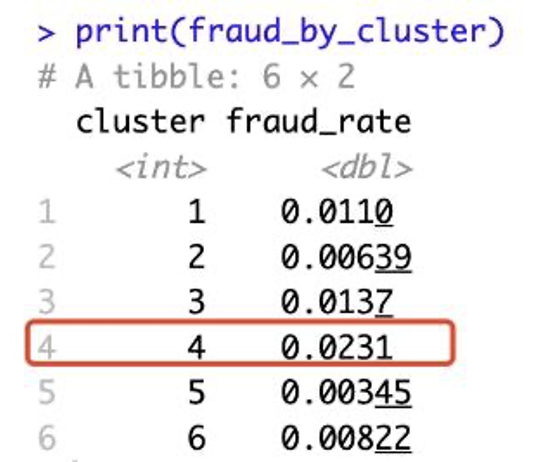
This table shows the rate of fraudulent transactions (fraud_rate) in each of the clusters that were identified in your k-means clustering analysis:

Cluster 1: Approximately 1.1% of transactions in this cluster were fraudulent.

Cluster 2: Approximately 0.64% of transactions in this cluster were fraudulent.

Cluster 3: Approximately 1.37% of transactions in this cluster were fraudulent.

Cluster 4: Approximately 2.31% of transactions in this cluster were fraudulent.

Cluster 5: Approximately 0.35% of transactions in this cluster were fraudulent.

Cluster 6: Approximately 0.82% of transactions in this cluster were fraudulent.

These rates represent the proportion of transactions that were marked as fraudulent within each cluster. For example, in Cluster 4, out of every 100 transactions, about 2.31 are expected to be fraudulent, based on this analysis. This is the highest rate among all the clusters, which suggests that transactions in Cluster 4 have a higher likelihood of being fraudulent.

Therefore, we might want to focus more resources on transactions from Cluster 4, as they seem to have a higher risk of fraud. For instance, these transactions could be subjected to additional checks or stricter control measures to prevent fraud.

Disconnect from Spark: The connection to Spark is terminated using the spark_disconnect() function.

Results

The application of clustering to identify potentially fraudulent transactions in our customer dataset can yield several notable benefits:

I. Enhanced Fraud Detection: By understanding the specifics of a transaction, the fraud detection functionality can be significantly improved. This helps us protect our business integrity and our customers’ financial interests more effectively.

II. Proactive Security Measures: If the system understands the specifics of a transaction, it can proactively flag suspicious activities, thereby potentially minimizing financial loss and increasing customer trust.

III. Insightful Data Analytics: This approach would allow our business to analyze transaction trends, identify patterns, and make more informed decisions related to customer behavior and fraud prevention.

IV. Automated Alert System: This model can assist in automatically flagging potentially fraudulent transactions based on the clusters formed, making the process more efficient and reducing the time to take necessary actions.

Recommendations

I. Credit Risk Score Analysis: Since there is a positive correlation between credit risk score and fraud, it is recommended to closely monitor accounts with higher credit risk scores for potentially fraudulent activities.

II. Age-Based Analysis: As there is a weak positive correlation between customer age and fraud, it might be beneficial to analyze the age distribution of customers involved in fraud to develop age-specific fraud detection strategies.

III. Address Verification: Given the negative correlation between previous and current address months count, it is advisable to incorporate address verification in the fraud detection process, especially for customers who have recently changed addresses.

IV. Session Management: The negative correlation between keep-alive sessions and fraud suggests that implementing robust session management strategies can potentially reduce the likelihood of fraud.

References

Bank account fraud dataset suite (NeurIPS 2022). (n.d.). Kaggle: Your Machine Learning and
Data Science Community.
https://www.kaggle.com/datasets/sgpjesus/bank-account-fraud-dataset-neurips-2022?select=Base.csv

Apache sparkTM - unified engine for large-scale data analytics. Apache SparkTM - Unified
Engine for large-scale data analytics. (n.d.). https://spark.apache.org/

Wei, T., & Simko, V. (2021). R package “corrplot”: Visualization of a correlation matrix (Version 0.90).https://cran.r-project.org/web/packages/corrplot/vignettes/corrplot-intro.html

SparkR (R on spark). SparkR (R on Spark) - Spark 3.4.1 Documentation. (n.d.).
https://spark.apache.org/docs/latest/sparkr.html

Javier Luraschi, K. K. (n.d.). Mastering spark with R. Chapter 2 Getting Started.
https://therinspark.com/starting.html#over

Google. (n.d.). Clustering algorithms | machine learning | google for developers. Google. https://developers.google.com/machine-learning/clustering/clustering-algorithms

Seif, G. (2022, February 11). The 5 clustering algorithms data scientists need to know. Medium. https://towardsdatascience.com/the-5-clustering-algorithms-data-scientists-need-to-know-a36d136ef68

Project Members:

• Xiaoge Zhang
• Yuchen Zhao